Smooth manifolds

This is an experimental venture by the LMS, in collaboration with Plus magazine, hoping to provide a wide range of readers with some idea of exciting recent developments in mathematics, at a level that is accessible to all members as well as undergraduates of mathematics. These articles are not yet publicly accessible and we would be grateful for your opinion on the level of the articles, whether some material is too basic or too complex for a general mathematical audience. The plan is to eventually publish these articles on the LMS website. Please give your feedback via the Council circulation email address.

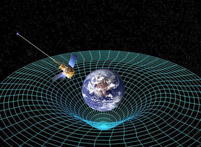
Massive bodies warp spacetime. Image courtesy NASA.

The Gromov-Hausdorff metric we explored in the previous articles lets us see compact metric spaces as themselves the points of a metric space. In this article we shall sketch two contexts where it is helpful to think of compact Riemannian manifolds as points of this space. The first is Einstein's general relativity, and the second is Perelman's proof of the Poincaré conjecture.

Newton's law of gravity says that each particle in the Universe attracts every other particle by instantaneous unmediated "action at a distance". This did not fit well with Maxwell's much later picture in which electric and magnetic attraction is mediated by the electromagnetic field. Later still the theory of special relativity made the idea of instantaneous interaction between distant particles completely untenable. Einstein had the wonderful idea that a gravitational field is a warping or curvature of space-time itself: its apparent action on particles is just the fact that they travel along geodesics in the curved manifold. His law of gravitation describes how the presence of matter produces the curvature of space-time. To put some flesh on this statement we need a digression about Riemannian manifolds and the description of curvature.

Riemannian manifolds

It is easy to imagine an $n$ -dimensional manifold $M$ smoothly embedded in the standard Euclidean space $\mathbb R^ N$ . We have a choice about which features of $M$ we want to regard as intrinsic, rather than just accidents of the way $M$ is embedded in $\mathbb R^ N$ . If we think of $M$ as a rigid object made of brass then the possible ways of embedding it in $\mathbb R^ N$ will differ only by rigid translations and rotations of $\mathbb R^ N$ . In that case the metric which $M$ acquires as a subspace of $\mathbb R^ N$ would be an intrinsic feature. At the other extreme, if $M$ were made of very elastic rubber then only its topology would be intrinsic. We get a Riemannian manifold if we make a choice intermediate between these two.

When $M$ is embedded in $\mathbb R^ N$ we can give it the metric for which the distance from a point $x$ to a point $y$ is the infimum of the lengths of all paths contained in $M$ which go from $x$ to $y$ . (The lengths of the paths are measured using the metric of $\mathbb R^ N$ .) By taking this metric as intrinsic we are choosing to regard $M$ as an object made of some flexible material which can be freely bent but not stretched, and can be embedded in Euclidean space in many different ways. A Riemannian manifold is simply a metric space which can arise in this way from a smooth submanifold of some $\mathbb R^ N$ . (This is the shortest but not the most useful – or the usual – way to give the definition.)

The tangent space $T_ x$ at a point $x$ of a smooth submanifold $M$ of $\mathbb R^ N$ is the n-dimensional vector subspace of $\mathbb R^ N$ formed by the tangent vectors – in the obvious sense – to $M$ at $x$ . But it is a striking fact that $T_ x$ is an intrinsic feature of $M$ as a Riemannian manifold. A tangent vector at a point $x$ can be defined intrinsically in terms of the metric space $M$ as an equivalence class of parametrized smooth paths through $x$ in $M$ , where two paths $f_0,f_1:(-\varepsilon ,\varepsilon ) \to M$ such that $f_0(0) = f_1(0) = x$ , both parametrized by distance from $x$ , are equivalent if the distance from $f_0(s)$ to $f_1(s)$ is of order $s^2$ as $s \to 0$ . (The condition that a parametrized path is smooth can also be expressed in terms of the metric of $M$ .)

In $\mathbb R^ N$ the length of a path $f:[a,b] \to \mathbb R^ N$ is given by

$\int _ a^ b \| f'(t)\| \ {\rm d}t.$

If the path lies in a smooth submanifold $M$ then the vector $f'(t)$ is a tangent vector to $M$ at the point $f(t)$ , so the metric of $M$ can be described very efficiently just by giving the lengths $\| f'(t)\|$ of all possible tangent vectors $f'(t)$ to $M$ – that is, by giving the inner product on each tangent space $T_ x.$ (In other words, instead of giving the lengths of all paths, we need only give the lengths of the infinitesimal paths.)

Among the intrinsic features of a Riemannian manifold are its geodesics. These are parametrized curves which minimize length between any two sufficiently close points on them. There is a unique geodesic emanating from any point $x$ of $M$ with any given tangent vector in $T_ x$ .

Curvature

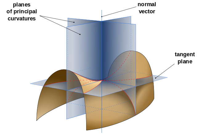
The curvature of a curve in the plane is the rate at which its direction changes when one travels along the curve with unit speed. This is entirely a property of how the curve sits in the plane. But things are more subtle for a surface in $\mathbb R^3$ . The natural way to describe the curvature at a point $x$ is to look at how the surface deviates from a flat plane – its tangent plane $T_ x$ . We can choose orthonormal coordinates $(u,v)$ in the tangent plane, and can describe the surface locally by its height $z$ above the tangent plane, that is, as the graph of a function $z$ from $T_ x$ to the line $N_ x \cong \mathbb R$ normal to the surface at $x$ . If we expand $z$ in a Taylor series at the origin, it will have the form

$z(u,v) \ = \ \frac{1}{2}L(u,v) \ + \ \ldots ,$

where $L$ is a quadratic form, and the dots represent terms of third order and higher. Thus the graph of $z = \frac{1}{2}L(u,v)$ is the paraboloid which best approximates the surface in the neighbourhood of $x$ .

The tangent planes and principal curvatures of a surface. (Image by Eric Gaba, CC-BY-SA)

If $\xi = (u,v)$ is a unit tangent vector at $x$ then $L(u,v)$ is the curvature of the geodesic through $x$ in the direction $\xi$ , or equally well – as in the figure above – of the curve in which the surface intersects the plane spanned by $\xi$ and the normal vector to the surface at $x$ . We can choose the coordinates $(u,v)$ so that $L$ takes the form

$L(u,v) \ = \ \kappa _1 u^2 + \kappa _2 v^2,$

so that the curvature of the geodesics emanating from $x$ varies between $\kappa _1$ and $\kappa _2$ as we rotate the direction in the tangent plane. We call $\kappa _1,\kappa _2$ the principal curvatures of the surface at $x$ . If they have the same sign the surface remains on the same side of its tangent plane, while if they have opposite signs the surface looks saddle-shaped at this point.

It turns out that part of the curvature of the surface is intrinsic. The product $K = \kappa _1\kappa _2$ , which is called the Gaussian curvature of the surface, is intrinsically defined because the area of a small disc of radius $r$ on the surface (which can be calculated just from the metric of the surface) is given by

$\pi r^2(1 - \frac{1}{12}Kr^2 + \mathcal O(r^4)). \ \ \ \ \ \ \ \ \ \ (*)$

A consequence of the Theorema Egregium is that the Earth cannot be displayed on a map without distortion. The Mercator projection, shown here, preserves angles but fails to preserve area. (Image by Jecowa, CC-BY-SA)

The fact that the product $K=\kappa _1\kappa _2$ is intrinsic is called Gauss's Theorema Egregium – his "remarkable theorem". It explains why we can bend a flat piece of paper to get a piece of a cylinder or of a cone (for which one principal curvature is zero at every point), but we cannot get a piece of a sphere.

To describe the curvature of a general Riemannian manifold $M$ of any dimension it is enough to understand the curvature of surfaces. If $\sigma$ is a (two-dimensional) plane in the tangent space $T_ x$ to $M$ at a point $x$ then the sectional curvature $K_ x(\sigma )$ is intrinsically defined as the Gaussian curvature at $x$ of the surface in $M$ swept out by the geodesics emanating from $x$ in all the directions in the plane $\sigma$ . To give $K_ x(\sigma )$ for all planes $\sigma$ in $T_ x$ is equivalent to giving what is called the Riemann curvature tensor of $M$ at $x$ .

The sectional curvatures $K_ x(\sigma )$ describe the intrinsic curvature of $M$ at $x$ completely, but there are cruder measures. The simplest is the scalar curvature, which tells us how the volume of a small ball compares with what it would be in Euclidean space. To be precise, the scalar curvature $R_ x$ at a point $x$ is defined by the property that the volume of a small ball of radius $r$ centred at $x$ is

$1 - \frac{1}{6(n+2)}R_ xr^2 + \mathcal O (r^4)$

times the volume of a ball of radius $r$ in Euclidean space $\mathbb R^ n$ .

A more refined measure is the Ricci curvature, which looks at the volume of the sliver of a small ball in each direction separately. It is a quadratic form $Ric_ x$ on the tangent space $T_ x$ . Its value $Ric_ x(\xi )$ on a unit tangent vector $\xi$ describes the volume of a narrow geodesic cone in $M$ with vertex $x$ , height $r$ , and axis in the direction $\xi$ as

$1 - \frac{1}{6(n+2)}Ric_ x(\xi )r^2 + \mathcal O (r^4)$

times the volume of the corresponding cone in the tangent space $T_ x$ .

The scalar and Ricci curvatures at a point $x$ can be read off from the sectional curvature: the scalar curvature $R_ x$ is the average of $K_ x(\sigma )$ over all planes $\sigma$ in the tangent space $T_ x$ , while, for a unit vector $\xi$ , the Ricci curvature Ric $_ x(\xi )$ is the average of $K_ x(\sigma )$ over the planes $\sigma$ in $T_ x$ which contain $\xi$ .

The Ricci curvature comes into play when you are considering manifolds of three or more dimensions. For a 2-dimensional manifold the Ricci curvature gives you the same information as the scalar curvature (Ric $_ x(\xi ) = 1/2 R_ x$ ). For manifolds of dimension 2 or 3 the Ricci curvature determines the curvature completely, but not in higher dimensions: a 4-dimensional manifold can have non-zero sectional curvatures even though its Ricci curvature vanishes.

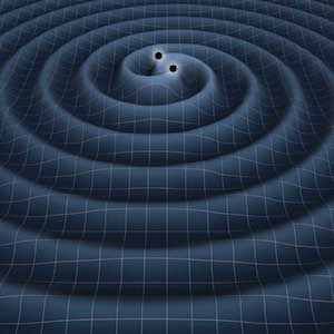
Gravitational waves travelling through empty space. (Image courtesy of NASA)

Gravitation according to general relativity

We might first guess that general relativity would require the curvature of empty space to be zero. But that would be too strong: Einstein's theory allows the possibility of gravitational waves – waves of curvature – travelling through empty space just as electromagnetic radiation does. The relativistic law is that only the Ricci curvature of space vanishes in the absence of matter. Just as classical physics tells us that the motion of particles in a fixed space-time is governed by a principle of least action, the vanishing of the Ricci curvature corresponds to a principle of least action for the Riemannian metric.

The variational principle in this case is that the total scalar curvature of any compact region of space-time (i.e. the integral of the scalar curvature over the region) is minimum – or at any rate stationary – with respect to variations of the metric in the interior of the region. When we make a small change $\delta g$ in the metric $g$ then the change in the total scalar curvature is described with the aid of a modification of the Ricci curvature, called the Einstein tensor. This is the quadratic form $E_ x$ on the tangent space $T_ x$ given by the difference

$E_ x(\xi ) \ = \ Ric_ x(\xi ) - \frac{1}{2} R_ x \ g_ x(\xi )$

between the Ricci curvature and $\frac{1}{2} R_ x$ times the quadratic form $g_ x$ (the Riemannian inner product on $T_ x$ ).

In fact the change in the total scalar curvature caused by the change $\delta g$ is the integral over the points $x$ of the space-time region of the inner product $\langle E_ x, \ \delta g_ x \rangle$ of $E_ x$ with the quadratic form $\delta g_ x$ . (The inner product used here between quadratic forms on $T_ x$ is induced by the inner product $g_ x$ on $T_ x$ .) Thus the variational principle for the total scalar curvature implies the vanishing of the Einstein Tensor; but the Einstein tensor vanishes if and only if the Ricci curvature does, except in the case of 2-dimensional manifolds, when $E_ x$ is automatically zero (as then Ricci curvature and scalar curvature are equivalent).

The least action formulation gives the clue to the general law of gravitation. The distribution of matter in space-time is described by the energy-momentum tensor. This is yet another quadratic form on the tangent space at each point: its value on a unit vector $\xi$ is the energy-density (per unit 3-dimensional volume) encountered by an observer whose trajectory in space-time has $\xi$ as its tangent-vector. Einstein's law of gravitation states simply that the Einstein tensor of space-time equals the energy-momentum tensor of the matter. The law expresses a principle of least action for the total action, which is the sum of the gravitational part (i.e. the total scalar curvature) and the usual non-gravitational action of the matter.

Evolving space-time

What is this telling us about how space-time evolves? For simplicity, let us suppose no matter is present. Space-time is a 4-dimensional manifold $M$ which we can imagine sliced up into 3-dimensional manifolds $\{ M_ t\}$ , where $M_ t$ is "space at time $t$ ". In Newtonian physics all the manifolds $M_ t$ are identical as point-sets, so that $M = M_0 \times \mathbb R$ ; but in Einstein's theory there is no God-given correspondence between points of space at different times. All the same, we can provisionally choose some identification of $M$ with $M_0 \times \mathbb R$ .

In terms of local coordinates $(x,y,z,t)$ chosen on $M$ , a Riemannian metric on $M$ is given explicitly by a symmetric $4 \times 4$ -matrix-valued function $g_{ij}$ of $(x,y,z,t)$ . (We have been avoiding mentioning that $M$ does not quite have a Riemannian metric: in fact the inner product on each tangent space is not positive-definite but has signature $(3,1)$ , with the "length squared" of a vector in the time direction being negative. Such metrics are called Lorentzian. Each time-slice $M_ t$ is nevertheless a genuine Riemannian manifold.) If the matrix-valued function $g_{ij}$ is given, together with its $t$ -derivative, when $t=0$ , we might naively expect the law of gravitation to determine how $g_{ij}$ evolves for $t>0$ . But actually that would not make sense: there cannot be an equation telling us how to calculate $g_{ij}$ for $t >0$ . For if we choose a different way of identifying $M_ t$ with $M_0$ , that is, we transport the metric by applying an arbitrary time-dependent diffeomorphism of $M_0$ which is the identity when $t$ is near $0$ , then we shall still have exactly the same Lorentzian manifold, but we shall have a quite different solution of the hoped-for equations, with the same initial conditions. The crucial physical fact is that the space of states of gravity in the absence of matter is the space of isomorphism classes of Ricci-flat Lorentzian manifolds and not the space of Lorentzian metrics on a given manifold. When we write $M = M_0 \times \mathbb R$ we are artificially giving points of 3-space a timeless reality which nature does not provide.

Among the valid ways of looking at the situation there is one which fits in well with the study of 3-manifolds via the Ricci flow, which will be our next topic. Having fixed on the initial time-slice $M_0$ – again a choice of our own making – we can choose to identify $M_ t$ with $M_0$ by moving with unit speed from a given point of $M_0$ along a geodesic in $M$ which is orthogonal to $M_0$ . When we do this, the metric on $M = M_0 \times \mathbb R$ is automatically of the form $\gamma _ t - dt^2$ , where $\gamma _ t$ is a varying Riemannian metric on the fixed 3-manifold $M_0$ . (Working on a fixed 3-manifold might seem to contradict what was said above, but in fact we have used up the invariance under diffeomorphisms of $M$ in choosing four of the ten components of the metric $g_{ij}$ of $M$ for our own convenience, leaving just the six components of $\gamma _ t$ to be determined.)

The point $\gamma _ t$ now moves like a "particle" on the infinite-dimensional manifold of all Riemannian metrics on $M_0.$ This is because, when we calculate the total scalar curvature of the metric on $M$ , we find it is of the form

$\int (T-V)dt,$

where $T$ , which we regard as the "kinetic energy" of the "particle", is a quadratic function of the "velocity" $\dot\gamma _ t$ at time $t$ , and $V$ is the total scalar curvature of the 3-dimensional metric $\gamma _ t$ , which we regard as the"potential energy".

Perelman and the Poincaré conjecture

Our last topic is the use of the Gromov-Hausdorff metric in Perelman’s proof of the Poincaré conjecture. This proof, which carried through a programme conceived by Richard Hamilton, amazed the mathematical world when it became known ten years ago. The conjecture is that any compact simply connected 3-dimensional manifold $M$ is diffeomorphic to a standard sphere in $\mathbb R^4$ . It is easy to show that the standard sphere is the only simply connected manifold with a metric of constant Ricci curvature, that is, Ricci curvature which is the same at every point and in every direction. That suggests trying to prove the conjecture by looking for a Riemannian metric on $M$ which minimizes "unevenness", in some sense, which is hard to pin down. Perelman’s method yields much more than the Poincaré conjecture: it elucidates the structure of all closed 3-manifolds.

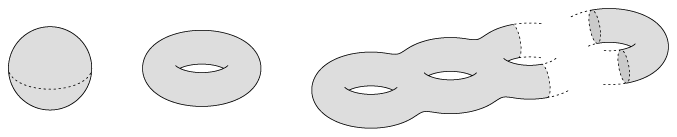
Two-dimensional surfaces are classified by their genus, or the number of donut holes that have been removed. A sphere is a surface of genus 0 and a torus has genus of 1, and so on. (Image by Daniel Müller from The Manifold Atlas Project')"

Let us begin with the simpler case of 2-dimensional manifolds – closed surfaces – and confine ourselves to the orientable ones. Then the topological classification is well-known: a surface is determined by its genus, or "number of handles". Furthermore, every surface can be given a metric of constant curvature, and that, in turn, implies the topological classification. If the constant curvature is positive the surface is a sphere, if it is zero the surface is a torus, and if it is negative we have a surface of genus $g \geq 2$ , constructed by identifying edges of a polygon in the hyperbolic plane with $4g$ sides, as described in an earlier section.

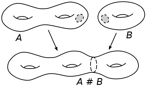
A connected sum of two 2-dimensional surfaces where a small ball (circle) has been removed from each and the boundaries of these sewn together. (Image by Oleg Alexandrov – CC BY-SA 3.0)

The topological classification of closed 3-manifolds (again supposed connected and oriented) is more complicated. The first step, however, is simple: every 3-manifold has a unique decomposition into prime factors under the operation of connected sum. The connected sum of two closed manifolds is formed by removing a small open 3-ball from each, leaving each bounded by a 2-sphere, and then sewing these 2-spheres together by an orientation-reversing diffeomorphism. This operation is – up to diffeomorphism – associative and commutative, and does not depend on where one removes the 3-balls from the manifolds.

The prime factors, however, can be decomposed further. Thurston proposed that the atomic 3-manifolds are those with a geometric structure: that is, those which admit a complete Riemannian metric of finite volume for which every sufficiently small ball is identical to every other ball of the same radius. According to his geometrization conjecture, which was finally proved by Perelman's work, each prime manifold can be cut along 2-dimensional tori into such geometric pieces. Thurston showed that in three dimensions there are eight different kinds of geometric structure: besides the constant curvature metrics of positive, negative, and zero curvature, which are characterized by the fact that all small balls are isotropic (i.e., they have the group of rotations SO(3) as their isometry group), there are five kinds which are not locally isotropic. Two of these are obvious: the manifold can be locally cylindrical, like the product of a line with a surface of constant positive or negative curvature; but there are also three exotic possibilities in which the manifold looks like a 3-dimensional Lie group, such as the Heisenberg group we met in article 2.

The details of Perelman's work are very long and intricate, but the geometric picture it gives us of how Thurston's geometric structure emerges is simple and beautiful. The picture starts with the space of isomorphism classes of compact Riemannian manifolds of a given dimension. This is a subspace of the space of all compact metric spaces, which has the Gromov-Hausdorff metric. The manifolds are not a closed subset of the space of compact metric spaces: a sphere of radius $r$ can shrink continuously to a point, or can shrink in all but one direction and become a 1-dimensional closed interval. We can also change the round sphere by shrinking its the equator so that it first becomes dumbbell-shaped, then pinches to a pair of spheres stuck together at one point, and then separates into two disconnected spheres: this too is a continuous path in terms of the Gromov-Hausdorff metric. But, of course, much worse things can happen.

Starting with an arbitrary Riemannian manifold, the strategy is to move it along a path in the space of manifolds so as to make its curvature more "even". It is not obvious how best to do this. Hamilton's insight was to focus on the Ricci flow: to move so that the rate of change of the inner product on each tangent space is -2 times the Ricci curvature at the point. (This defines a flow on the space of Riemannian metrics on a fixed underlying manifold, but it is equivariant with respect to diffeomorphisms of the manifold, so it induces a flow on the space of isomorphism classes.)

Why do we use the Ricci flow, rather than, say, the similar-looking gradient flow of the total scalar curvature, which is suggested by Einstein's equations? The reason is that the Ricci flow is essentially a nonlinear heat equation: its highest-order term tends to smooth out the metric by diffusion. The gradient of the Einstein action is not dispersive in this way – in fact, rather the opposite. We should not expect to be able to integrate it to define a flow on the space of Riemannian metrics.

In two dimensions the Ricci flow contracts the surface where the curvature is positive, and expands it where the curvature is negative. If we start with a dumbbell-shaped sphere the waist is expanded and the surface becomes progressively rounder. Once the sphere is positively curved everywhere the Ricci flow makes it smaller and smaller, so it is a good idea to combine the Ricci flow with an overall rescaling of the metric so that the total volume stays constant. It can be proved that any surface will then flow to one of constant curvature.

In three dimensions this does not happen. A three-dimensional manifold has waists which are 2-spheres rather than circles, and they are positively curved and contract to points in finite time, so that the manifold snaps into pieces: the first effect of the flow is to perform the decomposition of the manifold into its prime factors for the operation of connected sum. (We may, however, get a large number of 3-spheres splitting off, for these are identity elements for the connected-sum operation.) Once a component has snapped off it will continue to evolve under the Ricci flow, but we can rescale the components independently so that each has constant volume. If a component has positive Ricci curvature everywhere then Hamilton showed that it will evolve – after rescaling – to one of constant positive curvature. But, in general, large regions of negative curvature will emerge, separated by regions which will shrivel up but will not collapse completely in finite time. Each large region is bounded by a number of flat 2-dimensional tori, which become smaller and smaller under the rescaled flow. Each of the large regions tends to a manifold of constant negative curvature – a hyperbolic manifold – which has finite volume but has cusps: long narrow horns stretching out to infinity, whose cross-sections are 2-dimensional tori. (If one compactifies these by adding the points at infinity they will be singular points in the manifold, at which it looks locally like a cone whose base is a torus.) The existence of these cusps on most of the atomic 3-manifolds means that, like single oxygen atoms, they cannot occur uncombined in nature, that is, as compact 3-manifolds.

The final part of Perelman's proof is concerned with the shrivelling-up regions – bounded by tori – which remain when one removes the pieces which converge to hyperbolic manifolds. In the end, these too smooth out and acquire the more exotic geometric structures in Thurston's prophetic vision.

As a 3-manifold evolves under the Ricci flow some regions will collapse to singularities. To understand the topology of the initial manifold the crucial thing to establish is that no interesting topological feature is scrunched to a point and lost: in fact the only thing that happens topologically is that 2-spheres in the manifold contract to points in a standard way, performing the inverse of a connected-sum operation. That enables one to define the Ricci flow with surgery, which continues the Ricci flow through the singular times at which a sphere collapses. If we think of ordinary Ricci flow as analogous to flying a plane on autopilot then we need a human pilot to land the plane at each singular time, snip the singularity of the manifold away, and take off again.

The Ricci flow with surgery is a continuous path in the Gromov-Hausdorff metric which at isolated times leaves the class of smooth 3-manifolds. To construct it one needs precise control on what happens when the Ricci flow approaches a singular time. This is obtained by working in the space of 4-manifolds – "space-times" – swept out by a 3-manifold which is evolving under Ricci flow up to a time at which its scalar curvature becomes very large somewhere. It is in this space of 4-manifolds that one employs a version of the Gromov-compactness technique. More precisely, one studies a space of 4-manifolds equipped with a chosen point where the 3-dimensional curvature is large, and the idea is to consider a sequence of such space-times where the curvature at the chosen point tends to infinity as one goes along the sequence. One rescales the 3-dimensional metric of the $n^{\rm th}$ space-time by a large factor $\lambda _ n$ which will keep the curvature bounded, while simultaneously rescaling the time-parameter by $\lambda ^2_ n$ to preserve the Ricci-flow condition. A compactness result in the space of 4-manifolds enables one to extract a subsequence tending to a (non-compact) pointed space-time whose geometry is of a standard type which can be analysed in detail. The idea can be compared with the proof we sketched above of Gromov's theorem about nilpotent discrete groups, where by rescaling the word metric one found a sequence of pointed spaces converging to a Lie group – except that in that case the metric was being scaled downwards rather than upwards.

Add new comment