Solving crimes with maths: Busting criminal networks

Maths is often used in finding key criminals in organised crimes which involve many people, such as in terrorist attacks. This uses an area of maths called network theory, also known as graph theory. A network, or graph, is a structure used to model relations between objects. It consists of a set of nodes and a set of edges.

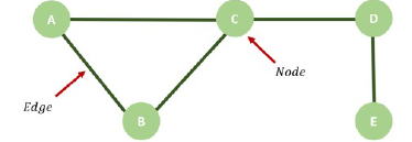
A network (or graph) with five nodes and five edges.

We can model the network of terrorists with the nodes representing terrorists and the edges representing connections between the terrorists. Investigators analyse social networks using the notion of centrality, aiming to identify the key players in the network.

Centrality is used to detect the relative importance of each criminal in the network. There are various measures of centrality that are commonly used to detect key players. Depending on the measure of centrality used, we may find different results when looking for the key criminal.

Degree centrality

Degree centrality measures how important a node is by counting the number of connections it has with other nodes in the graph. This is used to find popular players in the network.

$\mbox{Degree centrality of a node}=\frac{\mbox{Number of connections of that node}}{\mbox{Total number of nodes in the network -1}}.$

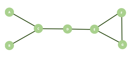
A network representing 7 criminals who have connections with each other.

We can apply this equation to the network above to calculate the degree centrality of criminal $C.$ Criminal $C$ is connected to 3 other criminals, criminals $A, B$ and $D.$ There are a total of 7 nodes in this network. So, the degree centrality of criminal $C$ is

$\frac{3}{7-1}=\frac{1}{2}.$

You can check for yourself that $E$ has the same value for degree centrality and that this happens to be the largest degree centrality in this network.

Betweenness centrality

Betweenness centrality measures how important nodes are to the flow of information in the network. It measures the flow of information through a criminal along the shortest path between two other criminals in a network.

In the table below we take every pair of criminals in our example network shown above, making sure we do not repeat any pairs. Information flowing from criminal $A$ to $B$ is the same as from $B$ to $A$ because we are looking at connections which have no direction.

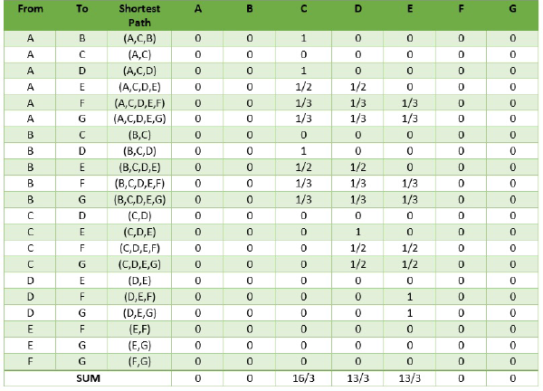
We then work out the shortest path between each pair of nodes (in a small network we can do this by inspection, but in a large one we can use Dijkstra's algorithm). The shortest path is the one with the smallest number of edges. Given a shortest path between two criminals, we then identify all the nodes that lie along it: these nodes will equally share a total score of 1 between them.

Here are some examples:

Looking at the pair $A$ and $B,$ we see that only criminal $C$ is on the shortest path between them, so $C$ is given a score of 1. No other criminals are on the shortest path from $A$ to $B$ , so all others get get scores of 0 for this pair.
If we look at the pair from $A$ and $C,$ we see that no criminals are on the shortest paths, so all criminals get a score of 0 for this pair.
Looking at the pair $B$ and $F,$ we see that we go through three other criminals on the shortest path between them. Since $C, D$ and $E$ are passed once and there are three criminals on the shortest path from $B$ to $F,$ the scores for $C, D$ and $E$ for this pair are all 1/3.

The betweenness centrality of a node is defined as the sum of all its scores. In our example, the betweenness centrality of criminal $C$ is $\frac{16}{3}$ , which happens to be the largest betweenness centrality score of all the criminals of the network.

(Strictly speaking, working out the betweenness centrality of each node also requires us to divide the result we get for a node from the procedure just described by

$\frac{(\mbox{total number of nodes in the network -1})\mbox{(total number of nodes in the network -2)}}{2}.$

However, this normalisation doesn’t change the order of criminals by their scores.)

Closeness centrality

Closeness centrality measures how easily nodes are reached in the networks. It detects criminals that are easily able to send information through a network.

To calculate the closeness centrality of a node $C$ , first write $N_1$ for the number of nodes that are one edge away from $C$ , $N_2$ for the number of nodes that are two edges away from $C$ , etc, up to $N_ k$ for the number of nodes $k$ edges away from $C,$ where $k$ is the longest chain of edges you can find starting at $C$ . The closeness centrality of $C$ is defined as:

$\frac{\mbox{Total number of nodes in the network-1}}{N_1+2N_2+3N_3+ ... +kN_ k}.$

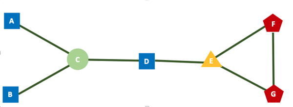
Our example network, modified to illustrate distance away from node C in terms of the number of edges.

As an example, suppose we want to find the closeness centrality of criminal $C$ in our example network. Criminals $A, B$ and $D$ are all 1 edge away from C and are illustrated with square shaped nodes. Node $E$ is 2 edges away from $C$ and shown as a triangle shaped node. Nodes $F$ and $G$ are 3 edges away from $C$ and are shown as pentagon shaped nodes. There are 3 nodes 1 edge away, 1 node 2 edges away, and 2 nodes 3 edges away from node $C.$ Substituting these values into our equation, the closeness centrality of criminal $C$ is:

$\frac{7-1}{1\times 3+ 2 \times 1 + 3 \times 2}=\frac{6}{11}.$

The way we define who is the most important criminal in the network matters. By using different measures of centrality to define the most important criminal, we may get different results. It may not necessarily be the person with the greatest number of connections who would be the key criminal in the network as we might initially think!

The maths you see in school or that you may study in the future is used in many areas of crime investigations which just goes to show how relevant maths is in the real world. There are many other exciting uses of maths in crime investigations, such as geographic profiling using Rossmo's formula and reconstructing accidents from skid marks which I encourage you to explore!

You may also want to read Solving crimes with maths: Bloodstain pattern analysis by Marcia Gomez.

About the author

Marcia Gomez is a recent Maths and Economics graduate from the University of Bath, who is particularly interested in statistics and how maths is used in the real world. She is currently applying her knowledge in the world of finance.