
Graphical methods III: the slugs bounce back
The story so far ...
It is 50 million years from now and the world, until recently, was dominated by slugs. Competing for land and resources, the slug world had divided into two rivalling superpowers, each threatening the other with a deadly arsenal of salty missiles. In Graphical methods I we saw how the slugs' fate hung in a dangerous balance — until all hell broke loose as each state launched its entire arsenal on the other. Very few slugs and other organisms survived. In Graphical Methods II we saw how those that did slowly started to take hold again and began to diversify.Imagine now that time begins to speed up, the Sun leaves the sky and returns, leaves and returns, until the passage of days is like the flickering of a strobe light. After a while, the Sun slows its eternal cycle through the sky until finally we're back on normal time. Many years have passed, clusters of robust slug buildings have emerged; fields are tilled. Basic economies and social cooperation have re-emerged. What can graphical methods tell us about the dynamics of these new, agrarian economies?
A slug farmer
Back to business
The slugs are now cultivating their staple crop, slimebubs. When they started, each slug family had its own patch of land on which to farm. Some were more successful, and had surplus to sell. While the days passed in the blinking of our eyes, professional farmers appeared, freeing up other slugs to become artisans of a different sort. These people needed to buy food from the farmers. The question we will address is how the demand for slimebubs from consumers relates to the amount of the crop produced by the farmers.
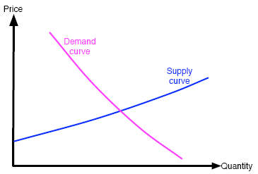
Figure 1: Supply and demand curves for slimebub production.
To approach this question, we need to talk about supply and demand curves. In figure 1 we plot two curves on axes of price against quantity. Although the background is more involved than we have the space for here, we can explain these two curves succinctly in the following way.
The supply curve shows how the quantity of slimebubs on the market depends on their price. If a point (x,y) lies on the supply curve, then this means that a slimebub price of y Slollars (the slug currency) per kilo will result in the farming industry producing x kilos of slimebubs in total. The farmers' decision of how many slimebubs to produce is of course very complex and does not only depend on their price, but when considering large numbers of farmers we can assume that they behave in this simple and easily predictable way. (Why this assumption is valid is part of the background detail which we cannot get into here.)
By contrast, the demand curve looks at things from the point of view of the consumers. A point (x,y) lying on the demand curve means that if the slimebubs cost y Slollars per kilo, then the total demand for slimebubs from all the consumers is x kilos. In other words, all the consumers taken together will buy x slimebubs in total. (Again, a typical consumer takes many things into consideration when deciding whether a price is fair and how much to buy, but a large number of consumers do act in a predictable, graphable way.)
Do the shapes of the curves make sense? The supply curve reflects a simple observation of human nature: if you can sell at a higher price, sell more and get richer. In this way, as price goes up, farmers produce more slimebubs so that they can reap even bigger incomes. So the supply curve will have the form indicated: it will increase, in other words it will have positive slope.
The demand falls as price increases because fewer people can afford or are willing to pay the higher prices. So the demand curve will decrease, it will have negative slope.
Slugs demand, slugs supply
A key point is that the demand curve determines the price — if the demand becomes low, then farmers are forced to reduce prices, and if it becomes high then farmers can increase them. The farmers try to supply to the demand in order to maximise their profits. One does not usually know the supply and demand curves in advance, but knowing their general shapes can give some insight into the world of commerce.
Slimebubs: nutritious and easy to grow.
Farmers naturally want to maximise their profits — they want to produce just the right quantity of slimebubs to meet the demand, and sell them at a price which is acceptable to them and ensures that the consumers will buy. As we will now explain, the point at which the supply and demand curves intersect gives us the equilibrium price and the equilibrium quantity. We have already talked about the importance of systems at or near equilibrium in Graphical methods II. In the case of the slimebub market, equilibrium means that the quantity purchased equals the quantity produced. It also gives the equilibrium price. Since at the equilibrium the amount sold is equal to the amount produced, the equilibrium price does not change. In fact, the equilibrium is the only point at which the system remains unchanged: if the farmers overproduce, then there is a slimebub surplus and the price drops, while if they underproduce then people become so eager to buy that farmers can charge what they like and the price goes up. Moreover, at equilibrium, the farmers are making a profit they deem acceptable and the consumer considers the price fair.
Finding equilibrium
Slimebubs, like many crops in our own day, are harvested just once a year. In such situations when there is a regular gap between each production round, reasonably regular price fluctuations can occur. Over the course of several years, how do these progress and what can this tell us about the stability of the equilibrium price?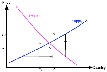
Figure 2: The cobweb model
To answer these questions we'll use a technique called cobwebbing, based on the following assumptions. In our simple model the demand curve determines the price, and the farmers aim to produce in the following year the amount on the supply curve which matches this price. Consider figure 2. The farmers produce a total quantity q1 of slimebubs in the first year of our analysis. Since the demand curve sets the price, they can charge a price p1 for each kilo of slimebubs. You can see that this price is lower than what they wanted to charge, a price given by their supply curve: they were losing money. Hence, the following year they will try to restrict their production to a level q2 which corresponds to the previous year's selling price. But in year 2, the quantity q2 will attract a price of p2. This year, the farmers are rolling in it (money, not slimebubs). This price then determines the target production levels for the following year, and so on. The shape we have drawn in solid black lines on the graph in figure 2 follows this reasoning. It looks like the beginning of a spider's cobweb, hence the name of this approach.
Remember that neither farmer nor consumer knows the actual shape of the supply and demand curves in advance, so they cannot simply agree to fix everything at the equilibrium values. However, the cobweb approach can help you guess the shape of the two curves from data collected as time passes: the demand curve contains all the points (qi,pi) (the quantity qi produced in year i and the price pi charged in year i), and the supply curve contains all the points (qi,pi-1) (the quantity qi produced in year i and the price pi-1 charged in year i-1). If you record the prices and quantities of slimebubs for a number of years, then you can mark the points (qi,pi) and (qi,pi-1) in a co-ordinate system. You can then fit curves that pass through the two sets of points, which approximate the demand and supply curves. Why not try using the Internet to find some data and plot some supply and demand curves of your own, using the cobweb model?
Stable markets
We can also use cobwebbing to answer questions of the stability of systems and the emergence of chaos. We don't have the space to talk about chaos here, but we can discuss the notion of stability. Suppose that the slimebub market is at its equilibrium point. We will say that the equilibrium of slimebub trading is stable if small deviations from the equilibrium point soon die out (the system returns to equilibrium) and unstable if this doesn't happen (if the price continues to fluctuate). Stability is a concept applied to other dynamical or changing systems, not just economics. A classic example is that of a balanced pencil. Both a pencil lying on its side and one balanced on its point are in equilibrium, since the situation is unchanging. However if you give the pencil on its point a little push, it will fall over, while the pencil lying down will not. The point-balanced pencil is in unstable equilibrium; the other in stable equilibrium.
Now draw two graphs on a piece of paper, and label the axes of each "price" and "quantity" as we have done below. On both graphs, draw a supply curve with the same gradient, or slope. Now on the first graph, draw a demand curve which is nearly flat, while on the second graph draw a demand curve which is very steep (both having negative gradients). Now comes the fun part. Turning to the first graph, pick a point on the demand curve close to the equilibrium point and begin your cobweb model from there. What happens? Now do the same for the second graph with the steep demand curve — what happens now?
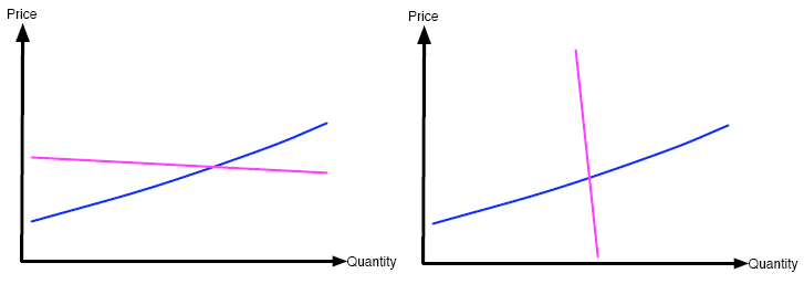
Figure 3: Draw a cobweb on each of these two graphs as described above. What is the difference?
Your conclusions could be summarised like this: the situation is stable when the negative of the demand curve's gradient is less than the gradient of the supply curve; unstable when the negative of the gradient of the demand curve is more than the gradient of the supply curve.
Thus, the comparison of gradients gives information on the stability of the market. But the gradient of each curve also tells us how sensitive supply or demand is to price. For example, when growing slimebubs is very sensitive to price, so that small changes in price result in big changes in production levels, then the supply curve is relatively flat (see figure 4). In this case, the negative of the demand curve's slope will almost always be greater than the slope of the supply curve because the latter is so small. As we've seen above, this gives rise to an unstable equilibrium, a worrying situation for the newly-emerging slug community to be in: prices are prone to start fluctuating unpredictably.
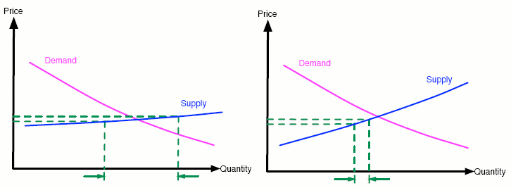
Figure 4: A comparison of a flat supply curve on the left and a steeper supply curve on the right. As shown, changes in price correspond to a larger change in quantity when the supply curve is flat.
If the slugs decide amongst themselves, in a form of government, to artificially fix production levels, then the supply curve becomes almost vertical (because the same amount is produced regardless of price). This changes the relationship between the negative slope of the demand curve and the slope of the supply curve, and can control the instability (see figure 5). In this case the equilibrium is reached automatically. Alternatively, the slug government may decide to fix the price of slimebubs, resulting in a horizontal demand curve. Again this forces the economy into equilibrium (see figure 6).
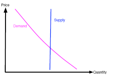
Figure 5: Artificially fixing production levels makes the supply curve almost vertical.
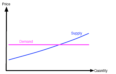
Figure 6: Artificially fixing the price makes the demand curve horizontal.
While it may seem like fixing prices and production levels will always stabilise markets and make everyone happy, we should remember that this only works under the following impossible conditions. All of the data which make up the supply and demand curves must be known in advance, and all producers and consumers must agree (or be coerced into agreeing) on prices and production levels. These conditions can never be met (and in the last case, never justly met) even with only one product on the market. Real economies have a vast number of products, and a consumer of one will be a producer of another. Wars have been fought on our planet over competing simplistic models of the market.
Back to the beginning
Assuming that the young slug communities manage to control instabilities in the market for their produce, we can happily expect them to grow and prosper. Before long, communities will merge into larger and larger groups, becoming more suspicious of their neighbours as competition for resources and control of their environment accelerates. A bit later, the development of their technological abilities begins to outpace that of their ethics. With slugkind's previous brush with annihilation now lost in a murky and distant past, Salty weapons are rediscovered, and not too soon after, redeployed. The cycle repeats. Will life always find a way?
About the author

Phil Wilson uses mathematics to understand how the skin of red blood cells works. The people he works with at the University of Tokyo hope that they can use this understanding to invent better ways of delivering medicine to the body. He is grateful to the editor of Plus for helping him channel his inner slug.
Comments
Anonymous
Hey thanks because of your example i was able to understand the cobweb model.