Bridges, string art and Bézier curves

The Jerusalem Chords Bridge

The Jerusalem Chords Bridge, Israel, was built to make way for the city's light rail train system. However, its design took into consideration more than just utility — it is a work of art, designed as a monument. Its beauty rests not only in the visual appearance of its criss-cross cables, but also in the mathematics that lies behind it. Let us take a deeper look into these chords.

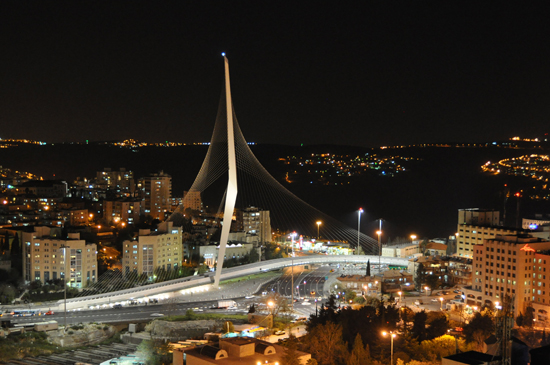
The Chords Bridge at night. Image: Petdad.

The Chords Bridge is a suspension bridge, which means that its entire weight is held from above. In this case, the deck is connected to a single tower by powerful steel cables. The cables are connected in the following way: the ones at the top of the tower support the center of the bridge, and the ones at the bottom support the further away sections, so that the cables cross each other.

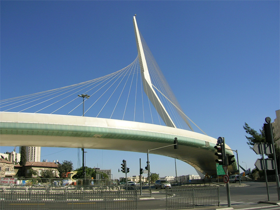
The Chords Bridge as seen from below.

Despite the fact that they draw out discrete, straight lines, we notice a remarkable feature: the outline of the cables' edges seems strikingly smooth. Does it obey any known mathematical formula?

In order to find out the shape the edges make, we are going to have to devise a mathematical model for the bridge. As the building itself is quite complex, featuring a curved deck and a two-part leaning tower, we will have to simplify things. While we lose a little accuracy and precision, we gain in mathematical simplicity, and still capture the beautiful essence of the bridge's form. Afterwards we will be able to generalise our simple description and apply it to the real bridge structure.

This is the core of modelling — taking only the important features from the real world, and translating them into mathematics.

Chord analysis

Let's look at a coordinate system, $(x,y).$ The $x$ axis corresponds to the base of the bridge, and the $y$ axis to the tower from which it hangs.

Figure 1: Coordinate axes superimposed on the bridge.

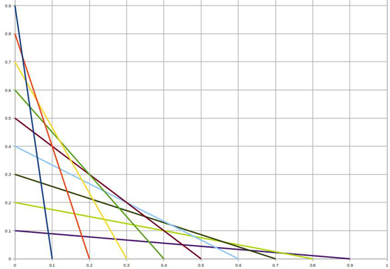
Taking the tower to span from 0 to 1 on our $y$ axis, and the deck from 0 to 1 on the $x$ axis, we make $n$ marks uniformly spaced on each axis. From each mark on the $x$ axis, we draw a straight line to the $y$ axis, so that the first mark on the $x$ axis is connected to the $nth$ on the $y$ axis, the second on the $x$ axis to the $(n-1)st$ on the $y$ axis and so on. These lines represent our chords. Let's also assume that the $x$ and $y$ axes meet at a right angle. This is not a perfect picture of reality, for the cables are not evenly spaced and tower and deck are not perpendicular, but it simplifies things.

Figure 2: Our axes with evenly spaced chords.

The outline formed by the chords is essentially made out of the intersections of one cable and the one adjacent to it: you connect each intersection point with the one after it by a straight line. The more chords there are, the smoother the outline becomes. So the smooth curve that is hinted at by the chords, the intersection envelope, is the outline you would get from infinitely many chords.

Forgoing the detailed calculations (which you can find here), we find that all the points on this curve have coordinates of the type

$(x,y)=(t^2, (1-t)^2)$

for all $t$ between 0 and 1. Hence:

$y(x)=(1-\sqrt{x})^2.$

Well, is this it? we ask. Is the shape going to remain an unnamed mathematical relation? In fact, no! While it is not easy to see at first, this is actually the equation for a parabola! To this you might reply that the equation for a parabola is:

$y(x)=ax^2+bx+c,$

which differs vastly from our result, and you would be correct. However, with a little work it can be shown that if we define $R = x+y$ and $S = x-y,$ we can rewrite our unfamiliar equation as

$R(S)=\frac{S^2}{2}+\frac{1}{2}.$

(See here for the details.)

And this indeed conforms to our well-known parabola equation. By replacing our variables $x$ and $y$ with $S$ and $R,$ we have actually rotated our coordinate system by 45 degrees. But this new coordinate system needn't frighten us. As we can see, the parabola equation is all the same.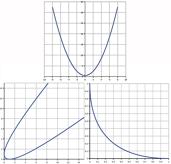

Figure 3: Top: The parabola R(S)=S²/2+1/2. Bottom left: The same parabola tilted by 45 degrees. Bottom right: Zoom on the square defined by x and y ranging from 0 to 1 in the tilted parabola, which is the region that represents the bridge.

The result we got — that the outline of the cables is essentially parabolic— is certainly satisfying, for the parabola is such a simple and elegant shape. But it also leaves us a bit puzzled. Is there a reason for this simplicity? Why should it be parabolic, and not some other curve? If we changed the shape of the bridge — say, to make the tower more leaning — how would it affect our curve? Is there any way in which we can make amends for our simplifications and assumptions that we had to perform earlier?

An unlikely answer

The answers to our questions originates from a surprising field: that of automobile design. Back in the 1960s, engineer Pierre Bézier used special curves in order to specify how he wanted car parts to look like. These curves are called Bézier curves. We shall now take a look at what they have to offer us.

We all know that between any two points there can be only one straight line; hence, we can define a specific line using only two points. In a similar fashion a Bézier curve is defined by any number of points, called control points. Unlike a straight line, it does not pass through all of the points. Rather, it starts at the first point, ends at the last, but does not necessarily go through all the others. Instead, the points act as "weights", which direct the flow of the curve from the initial point to the last.

The number of points is used to define what is called the degree of the curve. A two-point linear Bézier curve has degree 1, and is just an ordinary straight line; a three-point quadratic Bézier curve has degree 2, and is a parabola; and in general, a curve of degree n has n+1 control points.

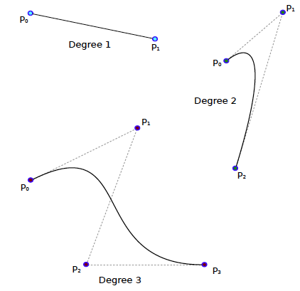
Figure 4: Bézier curves with degrees 1, 2 and 3.

A nice way of visualising the construction of a Bézier curve is to imagine a pencil that starts drawing from the first control point to the last. On the way, it is attracted to the various control points, but the level of attraction changes as the pencil goes along. It is initially most attracted to the first control points, so as the pencil starts drawing it heads off in their direction. As it progresses, it becomes more and more attracted to the later control points, until it finally reaches the last point. At any given time while we draw, we can ask: "what percentage of the curve has the pencil drawn already?" This percentage is called the curve parameter and is marked by t.

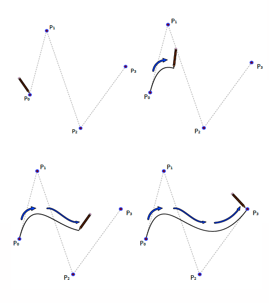
Figure 5: Drawing a Bézier curve.

How does all of this relate to our parabolic bridge? The connection is revealed when we take a look at how to actually draw a Bézier curve. One way of drawing it is to follow a mathematical formula that gives the coordinates of the curve. We will skip over that (you can have a look at the formula here) and instead move on to the second method: constructing a Bézier curve recursively. In this method, in order to construct an nth degree curve, we use two (n-1)st degree curves. It is best to illustrate this with an example.

Suppose we have a 3rd degree curve. It is defined by 4 points: $P_0,$ $P_1,$ $P_2,$ $P_3.$ From these we create two new groups: all points except the last, and all points except the first. We now have:

$\mbox{Group 1:} P_0, P_1, P_2$

$\mbox{Group 2:} P_1, P_2, P_3$

Each of these groups define a 2nd degree Bézier curve. Remember how we talked about using a pencil that moves from the first point to the last. Now, suppose that you have two pencils, and you draw both of these 2nd degree curves at the same time. The first will start from $P_0$ and finish at $P_2$ , while the second will start at $P_1$ and end at $P_3.$ At any given time during the pencils’ journey, you can connect their position with a straight line.

So, while these two are drawing, think of a third pencil. This pencil is always somewhere on the line connecting the two current positions of the other pencils and it moves along at the same rate as the other two. At the start it is on the line connecting $P_0$ and $P_1$ and since both pencils have moved along 0% of their curves, the third pencil has moved along 0% of this line, which puts it at $P_0.$ After the other two pencils have moved along, say, 36% of their curves and are at points $Q_0$ and $Q_1$ , the third pencil is on the line from $Q_0$ to $Q_1$ , at the point that marks 36% of that line. When the other two pencils have finished their journey, so they are at points $P_2$ and $P_3$ and have travelled 100% of the way, the third pencil is on the line from $P_2$ to $P_3$ at 100% along the way, which puts it at $P_3$ .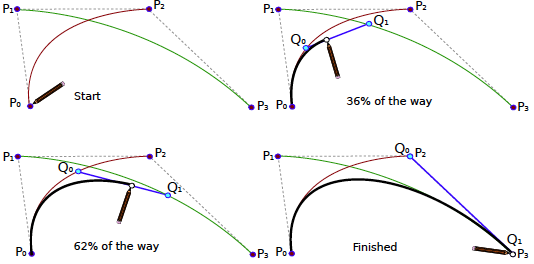

Figure 6: Building a cubic Bézier curve using quadratic curves. The red and green curves are the 2nd degree quadratic curves, while the thick black curve is the 3rd degree cubic - this is the curve we want to construct. The points Q₀ and Q₁ go along the two 2nd degree curves. Our drawing pencil always goes along the blue line connecting Q₀ and Q₁.

There is a very good question to be asked here. We have just described how to create an $nth$ degree curve, but doing so requires drawing $(n-1)st$ degree curves. How do we know how to do that? Luckily, we can apply exactly the same process to these assistant curves as well. We will build them out of two lesser degree curves. By repeating this process, we eventually reach a curve that we do know how to draw. This is the linear, 1st degree curve — it is just a straight line, which we have no problem drawing at all. Thus, all complex Bézier curves can be drawn using a composition of many straight lines.

Applying Bézier curves

Now that we are a bit familiar with Bézier curves, we can return to our original questions: what made the bridge's shape come out parabolic? How can we extend our model to fix the assumptions we made?

It turns out that our beautiful Chords Bridge is nothing but a quadratic Bézier curve! To see this, let’s go back to our coordinate system representing the bridge and draw a quadratic Bézier curve with the control points $P_0=(0,1)$ , $P_1=(0,0),$ and $P_2=(1,0).$ Using our recursive process the quadratic curve will be formed from two straight lines: the line from $P_0$ to $P_1$ (the $y$ axis from 1 down to 0) and from $P_1$ to $P_2$ (the $x$ axis from 0 up to 1).

Now suppose that the first pencil has travelled down the $y$ axis by a distance $t$ to the point $(0,1-t).$ In the same time the second pencil will have travelled along the $x$ axis to the point $(0,t)$ . The third pencil will therefore be on the line $L_ t$ from $(0,1-t)$ to $(t,0),$ $100 \times t$ % along the way. Thus, the Bézier curve meets all of the lines $L_ t$ for $t$ between 0 and 1. These lines (or at least $n$ of them) correspond to our bridge chords.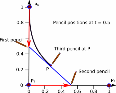

Figure 7: The red arrows represent the distance t travelled along the axes for t=0.5. The blue line is the line L_0.5.

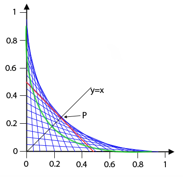
Now setting $t=0.5,$ we see that the half way point $P=(0.25,0.25)$ of the line $L_{0.5},$ lies on our Bézier curve. Figure 8 shows that $P$ also lies on the outline formed by the lines $L_ t$ . (See here if you're not convinced by the picture). This is enough to show that the Bézier curve and the outline are one and the same curve. As figure 8 shows, any other parabolic curve that meets all the $L_ t$ misses the point $P$ and crosses the line $L_{0.5}$ twice.

Figure 8: The blue lines represent some of the lines L_t. The red line is L_0.5. The green curve illustrates that any parabolic shape apart from the outline curve misses the point P.

Appreciating this fact allows us to deal with some of the previous model's inaccuracies. First, we assumed that the axes were perpendicular to each other, even though the tower and the deck of the bridge are actually at an angle. Now we see that this does not matter. The argument we just used continues to hold if we increase the angle between the axes by rotating the $y$ axis (and any other line radiating out from the point $(0,0)$ in between the $x$ and $y$ axes) anti-clockwise by the necessary amount. We know that any quadratic Bézier curve is a parabola, so the bridge outline is still a parabola. Second, we see that it does not matter whether the chords in our model are evenly spaced or not: they just represent some of the straight lines $L_ t$ whose outline define our Bézier curve. Third, the chords coming out of the tower do not span its entire length, but stop about halfway. This just means that we have to look at a partial Bézier curve. If we extend the deck onwards, we will still have a parabola, with $P_2$ as $(2,0).$ Then the outline of the chords is just the portion of the parabola that spans until $(0,1).$

Figure 9: The correct Bézier curve applied to the Chords bridge.

We can now rest peacefully, knowing the underlying reason to the parabolic shape of the Chords Bridge outline. Somehow, a curve that was used in the 1960s for designing car parts managed to sneak its way into 21st century bridges!

Béziers everywhere!

Bézier curves' abundance is far greater than just cars and bridges. It finds its way into many more fields and applications. One such field is that of string art, in which strings are spread across a board filled with nails. Although the strings can only make straight lines, a great many of them at different angles can generate Bézier curve outlines, just like the chords in the bridge do.

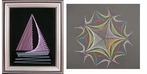
Figure 10: A boat and a pattern made from strings. Boat image from String art fun.

Another interesting appearance of Bézier curves is in computer graphics. Whenever you use the pen tool, common in many image manipulation programs, you are drawing Bézier curves. More importantly, there are many computer fonts which use Bézier curves to define how to draw their letters. Each letter is defined by up to several dozen control points and is drawn using a series of 3rd to 5th degree Bézier curves. This makes the letters scalable: they are clearly drawn and presented, no matter how much you zoom in on them.

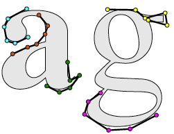
Figure 11: Some of the Bézier control points used to make "a" and "g" in the FreeSerif font (simplified).

This is the beauty of mathematics. It appears in places we would never expect and connects fields that appear entirely unrelated. Considering the fact that the curves were initially used for designing automobile parts, this is truly a display of the interdisciplinary nature of mathematics.

About the author

Renan Gross is an enthusiastic young scientist from Israel. He is interested in all fields of science, from mathematics and computer science to physics, informatics and biology. During his spare time he maintains a blog, plays the piano, and cycles fervently through the streets of Tel Aviv.

Comments

This is great!!! simply

This is great!!! simply ...keep em rolling in.......

Line Art Math

Thanks so much! I am doing line art in a math camp and couldn't quite get the equations together. Super work!

keep it up

good work

fantastic!

Really enjoyed this article, learnt a lot and it was very easy to read

Thank You!

I wanted information about the Jerusalem Chords Bridge, so I went to Wikipdia and saw a photgraph of the bridge. It is a beautiful structure, so I read the whole article in Wikipedia, including the footnotes; these footnotes include a link to your article. I am not a mathematician or scientist, but I still enjoyed reading your explanation of the shape of the bridge. Thank you.

Thank you for this article it

Thank you for this article it has been very helpful in an assignment I had to do on the applications of Bezier Curves.

Fun reading about Beziers

The way you had interlinked the Jerusalem bridge to a parabolic curve to a bezier curve and your description of how to create Bezier curves, fantastically presented! Loved reading the article

Jerusalem Bridge

Hi, great article.

I was wondering though, do you believe with these straight lines forming the Bezier curve, that it in fact structurally holds up the bridge?

Such an odd shape and if you study the construction the sequence doesn't quite make sense. The cables are attached to the side the bridge as opposed to the centre?

Do these cables really hold up the bridge? Or is it an illusion?

Adjusting cable tension - how ?

Sydney's Anzac Bridge -- many pix - e.g., http://sydneynearlydailyphot.blogspot.com.au/2011/02/anzac-bridge-from-… is far simpler - though there are interesting views where the lines from the two towers can be seen crossed. This may be more of an engineering question -- but I wonder just how the load in the cables is adjusted so the bridge is properly supported? And with increasing traffic load - why is the tension still properly shared ?
An issue for the Jerusalem Chord bridge too - though with much lighter traffic loads -- but very concentrated point load as a light rail crosses.

Harvey

Plus.Maths.org