Spontaneous spirals
Spirals are common in nature. We've all admired the beautiful spirals that occur in sea shells, we can find spirals in plants, and even in the arms of galaxies or weather patterns. There are also situations in which spirals aren't a result of slow growth, but occur spontaneously in biological or chemical systems. A famous example from chemistry is the Belousov-Zhabotinsky (BZ) reaction: when several chemicals are mixed together in a petri dish, the resulting solution forms changing spiral patterns, as seen in this video:
In biology a particular slime mould, called dictyostelium discoideum, gives rise to similar patterns. The organism normally lives as individual amoebae that consist of a single cell. The spirals arise when these single-celled amoebae aggregate into a body made up of many cells, which then produces spores that develop into individual amoebae again.
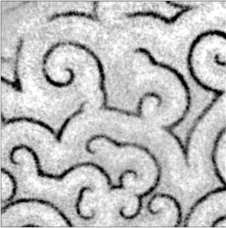
Spiral waves in dictyostelium. Image from Regulation of Spatiotemporal Patterns by Biological Variability by Miriam Grace and Marc-Thorsten Hütt. Published in PLOS Computational Biology, reproduced under Creative Commons.
What's remarkable about both these examples is that there is no single unit, or even a small group of units, that controls the behaviour of the system as a whole and "dictates" the formation of the spiral patterns. Instead, the individual units interact only locally with whatever other units happen to be nearby. Yet, despite this lack of a central control and the limitation to local interactions only, these systems produce global patterns, such as the spiral waves. They also produce coordinated behaviours, such as aggregating into one multi-cellular body, that are at the scale of the system as a whole, well beyond that of a single individual.
These are examples of decentralised spatial systems. But how do their patterns form?
Cellular automata
Spontaneous spiral wave formation in decentralised spatial systems can be reproduced and studied with simple mathematical models known as cellular automata. A cellular automaton (CA) consists of a large number of similar individual units ("cells") arranged in a particular way. For example, the cells could be squares that line up in a row (a one-dimensional arrangement) or they could form a two-dimensional grid, like graph paper.
Each cell in this grid contains a variable that has one of a number of possible values, for example either 0 or 1. The values of these variables can be visualised by simply colouring each cell accordingly, such as white and black for 0 and 1. The variables could also take as values numbers between 0 and 1, in which case we can use or a colour gradient to represent them.
At regular time steps, each cell updates the value of its variable according to a given mathematical formula that takes account of the current values of the cell itself and those directly surrounding it. For example, the formula might decree that a cell that currently has the value 0, and whose neighbours also all have the value 0, will change its value to 1. Thus, at each time step, the colours of the cells in the grid change accordingly, which gives rise to a constantly changing visual pattern in the system as a whole. However, there is no central control in the system, and each cell only interacts with its closest neighbours.
The simplest version of a CA consists of a row of cells whose values can only be 0 or 1. The new value (or colour) of a cell depends only on the cell itself and one neighbour on either side, that is, a three-cell local neighbourhood. This is known as an elementary cellular automaton (ECA). In this case, the update formula can simply be represented by a lookup table that lists each of the possible triples of values that represent a local neighbourhood, together with the new value of the centre cell for each of these configurations. Since each cell can takes one of two values, there are 23=8 possible triples. An example is shown in the table below.
| Neighbourhood | 000 | 001 | 010 | 011 | 100 | 101 | 110 | 111 |
| New value of middle cell | 0 | 1 | 0 | 0 | 1 | 0 | 0 | 0 |
In this example (which is known as ECA 18) a string of cells that consists of a single 1 and the rest 0s , that is,
| ... | 0 | 0 | 0 | 0 | 1 | 0 | 0 | 0 | 0 | ... |
at the next time step changes into the following string:
| ... | 0 | 0 | 0 | 1 | 0 | 1 | 0 | 0 | 0 | ... |
Which at the next time step changes into:
| ... | 0 | 0 | 1 | 0 | 0 | 0 | 1 | 0 | 0 | ... |
This process of updating the cells according to the rule can be continued indefinitely.
Replacing the numbers by colours (black for 1 and white for 0) and placing the strings, as they evolve at each time step, underneath each other gives the space-time diagram of the ECA.
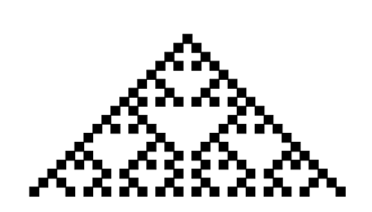
ECA 18 starting from a row with only one back cell (top). The picture shows the rows you get from 18 time steps.
A different starting string will give a slightly different picture, but retain some of the overall patterns. Here is the diagram for a starting string in which the colour of each cell has been chosen at random.
ECA 18 starting from a random string (top).
The global patterns, even though generated by a simple and local update formula, look very natural. These patterns resemble, for example, ones that occur on sea shells.
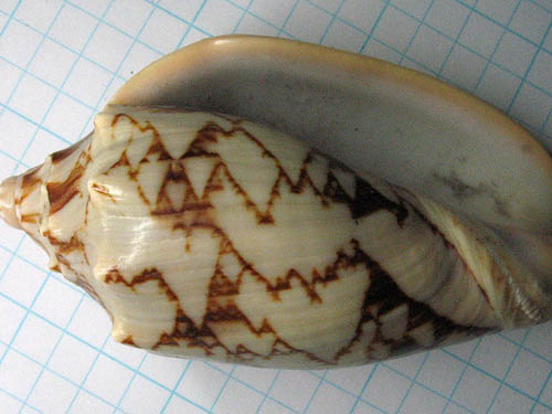
Image: tehsma, CC BY-NC 2.0.
Note that the new cell values in an ECA, that is the 0s and 1s in the bottom row of the lookup table above, could have been assigned in any way. There are two possible values for each of the eight triples, giving rise to 28=256 different possible lookup tables for ECAs. The particular patterns that show up in a ECA's global dynamics depend on which of these lookup tables is used. You can see a picture of each ECA on Wolfram Mathworld.
Spiral waves
The ISCAM model for spiral waves
For the ideal storage model imagine a container that contains a certain amount of a substance. At regular time intervals a proportion $R$ of the substance is released from the container, and a fixed amount $C_s$ is replenished. If the amount of the substance in the container is $S$ at the current time step, then it will be $$S^{\prime} = S - RS+C_S$$ at the next time step. The release proportion is itself dynamic, depending on the amount released at the previous step. If the proportion was $R$ at one time step, then the release proportion $R^{\prime}$ for the next time step is $$R^{\prime} = \frac{1}{1+e^{-5RS+C_r}},$$ where $C_r$ is a fixed constant. The two parameters, $C_s$ and $C_r$ can be tuned to change the dynamical behaviour of the model. Now imagine this dynamical system running separately in each individual cell of a 2D CA. In other words, each cell in the CA now contains two variables: $S$ and $R$. However, instead of each cell updating its variables in isolation, there is a coupling between neighbouring cells, as there needs to be for the system to form a CA. Write $R_i$ for the release proportion of a given cell at the current time step. First, calculate the average of the $R$ values of the eight neighbours of the given cell. Let's write $R_A$ for this average. Next, for a fixed value $p$ between 0 and 1 calculate $$\bar{R_i} = (1-p)R_i+pR_A.$$ Now, each time the cell calculates its new values $S^{\prime}$ and $R^{\prime}$, using the ISM formulas given above, its current $\bar{R_i}$ value is used instead of $R_i$. This way, the dynamics of each cell is coupled to that of its direct neighbours. The additional parameter $p$ (between 0 and 1) determines the strength of this coupling. If $p=0$ there is no influence of neighbouring cells on the new values $S^{\prime}$ and $R^{\prime}$ in a given cell. When $p=1$ there is complete influence.To generate spiral waves with cellular automata, we need to use a somewhat more elaborate version of a CA. First, a two-dimensional space is needed. This means that the CA now consists of a 2D regular grid, where the new value of each cell is determined by the cell itself and its eight directly surrounding neighbours.
Next, instead of just using the two possible values 0 and 1, a continuous range of values is needed, for example the real numbers between 0 and 2. Finally, a more sophisticated update formula is needed.
The particular update formula we will use here is based on the so-called Ideal Storage Model (ISM). Imagine that each cell in our 2D grid is a container that contains a certain amount of a substance. At regular time intervals a certain proportion of the substance disappears from the cell, and a fixed amount is replenished. The proportion that disappears depends on the amount of substance that disappeared from the cell at the previous time step, but it also depends on the proportion that disappeared from the eight neighbouring cells at the previous time step (see the box for the precise rule). In this way, the amount of the substance in each cell varies over time in a way that depends on its eight neighbours and the past. The amount is represented by a number between 0 and 2, which in turn can be represented by a colour from black (for a zero amount) to bright red (for an amount value equal to 2). This embedding of the ISM in a 2D CA is known as the Ideal Storage Cellular Automaton Model (ISCAM).
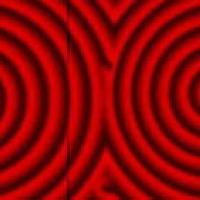
The ISCAM is capable of generating spontaneous spiral waves very similar to the ones observed in our two examples at the beginning of this article, the BZ reaction and dictyostelium. The figure below shows several selected time steps from one particular run of the ISCAM on a 100x100 grid, starting from a purely random initial configuration, and with parameter values $C_s=0.5$, $C_r=2.5$, and $p=0.2$ (see the box above to see how these parameters influence the ISCAM). The different shades of red represent the amount $S$ of the substance in each cell, with black denoting $S=0$, bright red $S=2$.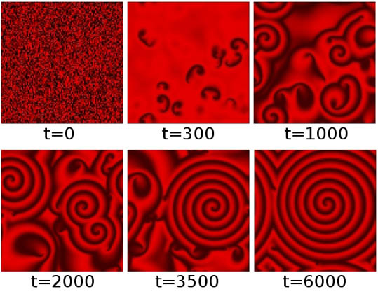
One particular sequence of global patterns generated by the ISCAM in a regular grid of 100x100 cells. The system starts (at t=0) with completely random values in the cells. These values are colour-coded with a gradient from black (S=0) to bright red (S=2). After 300 time steps (t=300), several "nucleation sites" start to appear, which then grow into real spirals (t=1000) that start to interact (t=2000) and compete (t=3500) with each other, until eventually one spiral dominates the system (t=6000).
There is a small problem when working out the behaviour of the ISCAM on a finite grid: in order to work out what is happening in the cells on the edge of the grid, we need to know what is happening in the cells that are their neighbours, but which aren't on the grid and for which we haven't got any values. To get around this problem, we simply wrap the grid around so that the cells in the leftmost column and the rightmost column are considered each other's neighbours, and similarly for the top and bottom rows. In other words, the CA grid actually exists on a doughnut shape (or torus) which is what you get when you glue together opposing sides of a square.
The one-minute movie below shows a similar run of the ISCAM in real time, using the same parameter values as in the figure above. Click the "play" button to start the movie.
It turns out that these spirals are remarkably robust. For example, when a perturbation ("noise") is introduced in a spiral by resetting the $S$ values in a 3x3 block of cells to zero (black), and the system is then allowed to proceed, the spiral will simply continue to go around, quickly removing the perturbation, seemingly as if nothing ever happened. This process is shown in the figure below on a 50x50 grid.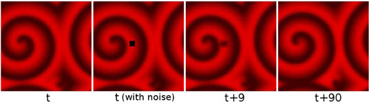
Noise (the black square) is introduced into the system at a given time t. After nine time steps (t+9) the spiral has gone around once, and the noise is reduced to a vague smudge. After 90 time steps (t+90) everything looks just as before.
Natural systems tend to produce many beautiful and often complicated patterns. However, as the above example shows, the underlying mechanisms and mathematical principles can be surprisingly simple. Using a basic mathematical model (a cellular automaton with an update formula based on the ISM), spontaneous spirals in spatial systems cannot only be accurately reproduced, but also studied and understood in more detail. This certainly makes for some interesting psychedelic science!
Acknowledgements
The author would like to thank his former colleagues Andreas Dress, Lin Wei, and Peter Serocka (at the Partner Institute for Computational Biology, Chinese Academy of Sciences, and the Centre for Computational Systems Biology, Fudan University, Shanghai), with whom the ISCAM was originally developed.
About the author

Wim Hordijk is a computer scientist currently on a fellowship at the Konrad Lorenz Institute in Klosterneuburg, Austria. He has worked on many research and computing projects all over the world, mostly focusing on questions related to evolution and the origin of life. More information about his research can be found on his website.
Comments
JT
Nice article!
BTW: an online-visualization can be found here:
https://www.shadertoy.com/view/XtcGD2
(or google shadertoy Belousov–Zhabotinsky reaction),
simulated on the GPU.