Phantom jams
Traffic jams are a pain, especially when they happen for no apparent reason. Even when a road is only moderately full and there are no obstacles up ahead, traffic can bunch up, slow down, and even come to a complete halt. Traffic researchers have long been interested in such phantom jams — and mathematical models can tell us why they happen.

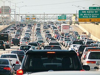
Rush hour on IS 95 in Florida. Photo: B137, CC BY-SA 4,0.
You can build a model based on the simple assumption that drivers vary their speed according to the distance between themselves and the vehicle in front. If the distance decreases because the car in front brakes, a driver will slow down. If the distance increases, a driver will speed up until they reach the speed they desire (or the speed dictated to them by a speed limit). This is exactly what happens in reality.
To keep things simple let's also assume that we have a number of cars travelling in a single lane around a ring. This is less realistic but means we can assume that the number of cars on the road stays the same, which makes for easier maths.
It's relatively straight-forward to capture this situation using mathematical equations that express the acceleration of each car in terms of the headway in front of them and their current speed (see below for some details). Given an initial speed and distribution of cars, the solutions to the equations will tell you how fast the cars will be travelling at any given time.
This toy model is so simple, you'd expect the traffic to settle down into an even flow going round and round the ring. Car-following models like this do indeed predict just that: there is a uniform flow equilibrium, which is stable in the sense that little variations in speed won't knock the equilibrium off kilter. That's exactly the kind of situation we'd want in real life, but we all know that in reality things can play out very differently.
Chain reaction
One crucial thing the model is missing is the fact that drivers aren't machines: while driving along they might be fiddling with the radio, talking to the kids on the back seat, or arguing with the satnav. In short, drivers don't react immediately to a change in the distance to the car in front. A little delay in their reaction could make quite a difference to how hard they need to brake.
We can add this fact into the model by including a reaction time delay parameter. When you do this, the dynamical system does indeed change its overall nature: apart from the stable uniform flow behaviour, the equations now also admit a stop-and-go wave that can persistently travel down the road in the opposite direction of the traffic flow, even if the density of traffic isn't all that bad. The crucial ingredient here are the drivers' delayed reactions to even minor disruptions of traffic, such as a lorry ahead changing lanes. It's those delays that can trigger the stop-and-go wave. Our simple model has therefore delivered an explanation for phantom jams that previously wasn't obvious.
Traffic jam waves spreading backwards through the traffic have been predicted by other mathematical traffic models too. They have even been observed in a real-life experiment which reconstructs the simple set-up we described above: it had 22 cars travelling around a ring at a constant speed of roughly 30kmh and even though traffic started out flowing smoothly, jam waves were soon triggered by little variations in speed.
The good thing about mathematical models of traffic is that they can not only explain baffling phenomena, but also help us decide how to avoid them. The simple model above suggests that keeping your reaction time to a minimum can do more to avoid jams than you might think — perhaps driverless cars will help in this context. But models can also be used to figure out how things such as variable speed limits may help guide traffic out of a jam and back into uniform flow. The roads of the future should, and hopefully will, be built on maths.
A traffic model
Suppose there are $n$ cars and write $v_i(t)$ for the velocity of car $i$ at time $t$. Write $h_i(t)$ for the distance between car $i+1$ and car $i$ at time $t$ so $h_i$ is the headway of car $i$. Then $h_i(t)$ should satisfy $$dh_i(t)/dt = v_{i+1}(t)-v_i(t),$$ capturing how the headway between two cars changes as a result of the cars' changes in velocity. In an optimal velocity model the acceleration $dv_i(t)/dt$ of car $i$ is described by the differential equation $$dv_i(t)/dt =\alpha\left(V(h_i(t))-v_i(t)\right),$$ where $\alpha$ is a parameter called the sensitivity and $V(h_i(t))$ is a function that represents the optimal velocity for a given amount of headway. $V(h_i)$ could be any type of function that satisfies certain realistic conditions. For example, as the headway $h_i$ in front of a car increases, the optimal velocity $V(h_i)$ should also increase until it reaches the legal speed limit, reflecting that drivers want to speed up when they can. The equation above shows that if the velocity $v_i$ of car $i$ is smaller than the optimal velocity $V(h_i)$ then the driver will accelerate, if it is larger then the driver will brake, and if the two are equal the drive will do neither. (In both of the equations above, if $i=n$ we take $i+1$ to be $1$, reflecting the fact that cars are travelling around a ring.) As it stands, the second equation means that drivers react to a change in their headway instantaneously by breaking or speeding up. But we can also include a reaction time $T$ to get the equation $dv_i(t)/dt =\alpha\left(V(h_i(t-T))-v_i(t)\right).$$You can find out more in this paper by Gábor Orosz, R. Eddie Wilson, and Bernd Krauskopf or this one by Gábor Orosz and Gábor Stépán.
About this article

This article is based on a chapter from the new book Understanding numbers by the Plus Editors Rachel Thomas and Marianne Freiberger.