Plus Advent Calendar Door #16: Calculus

One thing that will never change is the fact that the world is constantly changing. And thanks to the tools of calculus, we can mathematically capture change which helps us to understand the world we live in.

There's two sides to calculus: differentiation describes how fast things change and integration describes how fast things add up.

Differentiation

A good first example of differentiation is finding the rate of change of a function by considering the slope of the function's graph. For example, a straight line, described by the equation $y=mx + c$ , always has a gradient of $m$ , no matter where you are on the $x$ -axis. So the rate of change for the value of $y$ (the amount by which $y$ changes as you vary $x$ ) will always be $m$ .

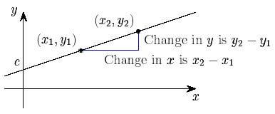
The gradient of a straight line

But what about the curve $y=x^2$ ? Near to $x=0$ the value of $y$ changes slowly, but it changes faster and faster as $x$ moves further away from zero.

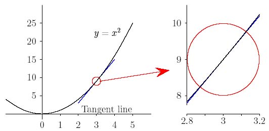
Finding the gradient of y=x<sup>2</sup> at x=3

If you zoom in on a smooth function, like y=x² it looks very similar to the flat tangent line at that point.

If you have a smooth function, one that up close can be approximated by a flat, tangent line, you can calculate the rate of change of the function as the gradient of the tangent line at any point on the curve. Differentiation allows us to calculate the value of this gradient at any point for such a smooth function.

You can approximate the gradient of your curve $y=f(x)$ by drawing a straight line from the point $(x,(f(x))$ to a very nearby point on the curve, and calculating the gradient of that straight line.

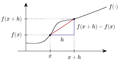
Calculating the gradient of a general function

For example for our function $f(x)=x^2$ , and a very small number $h$ , we calculate that the gradient of that straight line is

$\frac{f(x+h) - f(x)}{h} = \frac{(x+h)^2 - x^2}{h} = \frac{x^2+2xh+h^2 - x^2}{h} =2x+h.$

If we think about what happens as $h$ gets very small indeed (but is still nonzero), the slope of this line will be very close to the slope of the tangent line at the point $(x, f(x))$ . By a limiting argument, which can be made watertight mathematically (you can read more about how that's done here), we say that the function $f(x)=x^2$ has a tangent line with gradient $2x$ . This is the derivative of the function, giving the gradient of the tangent line at any point.

You can see the full details of how to differentiate this way, by calculating gradients of graphs of a function, in Making the grade. But the full power of calculus is unleashed when you move to differentiating by manipulating the algebraic expressions that describe these functions. Then you can use a whole tool box of rules (you can see some examples below) to help you differentiate any smooth function. You can see all these rules and why they work in Making the grade: part ii.

If you use maths to describe the world around you — say the growth of a plant, the fluctuations of the stock market, the spread of diseases, or physical forces acting on an object — you soon find yourself dealing with derivatives of functions. The way they inter-relate and depend on other mathematical parameters is described by differential equations. These equations are at the heart of nearly all modern applications of mathematics to natural phenomena. The applications are almost unlimited, and they play a vital role in much of modern technology. (You can read more in Maths in a minute: Differential equations.)

Integration

Integration describes how change accumulates, which you can calculate by adding up infinitely many infinitely small things. For example, let's consider how the area under the graph $y=x^2$ increases as $x$ increases from 0.

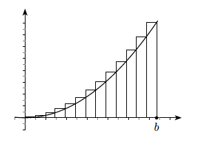
One approach to calculating the integral for our example $y=x^2$ between $x=0$ and $x=b$ , is by using a sequence of $n$ rectangles to approximate the area between the curve, the $x$ -axis and the vertical line at $x=b$ . The rectangles divide the $x$ -axis into intervals of length $b/n$ . The height of each rectangle is the maximum value of the curve on the corresponding interval. Then you can write the approximate area as the sum of these $n$ rectangles.

The more rectangles you use – the more finely you slice the area – the closer your approximation gets to the actual area. So just as we used a limiting argument to calculate the tangent of a curve, you can take the limit of this sum of rectangles as you increase the number $n$ , to give you the integral of the function.

For our example of $y=x^2$ , this process calculates that the area between the curve and the x-axis, from 0 up to the vertical line at $x=b$ , is $\frac{b^3}{3}$ .

You can see the details of this limit approach in Intriguing Integrals. Before Isaac Newton's discovery of the fundamental theorem of calculus, which allows integrals to be evaluated in practice as anti-derivatives, resorting to such sums was the only way to calculate integrals as areas.

Using this algebraic approach we find that the integral of the function $y=x^ k$ is $\frac{x^{(k+1)}}{(k+1)}$ , and is written

$\int x^ k\mathrm{d}x = \frac{x^{k+1}}{k+1} +c.$

(You'll notice a constant $c$ has appeared. This is called the constant of integration, and appears if you haven't defined the interval over which you are integrating.) You can see that if we differentiated this integral, $\frac{x^(k+1)}{(k+1)}$ , we would get back to our original function $x^ k$ (notice that $c$ disappears with differentiation). You can find out more about this approach of integrating algebraic expressions in Intriguing integrals: part ii.

Not everything is solved by calculus

Isaac Newton

We have Newton and Gottfried Wilhelm von Leibniz for the development of calculus as a systematic set of tools. But this definitely wasn’t a joint project and their independent discovery led to one of the more famous disputes in maths.

Both men worked on calculus in the second half of the seventeenth century. Pulling together various bits and pieces, and adding their own ingenious contributions, both succeeded in bringing structure into the jumble of ideas that had been calculus up to that time. Newton developed his method of fluxions, as he called it, a few years before Leibniz developed his theory, but Leibniz's work was published first. Leibniz had not been aware of Newton's work, and had approached the subject in a completely different way, but this didn't stop Newton from accusing Leibniz of theft.

Gottfried von Leibniz

Corresponding mostly via third persons, learned journals and pamphlets, Leibniz continued to protest his innocence and Newton continued to vent his wrath. Newton indignantly claimed that "not a single previously unsolved problem was solved" in Leibniz's work. Leibniz called a Newton supporter an idiot. A Royal Society commission was set up to arbitrate, but was completely biassed towards Newton and unsurprisingly found in his favour. The author of the commission's final report was none other than — Newton himself!

The controversy over the true inventor of calculus was never resolved in the men's lifetime and overshadowed the end of both their lives. For Newton this was not the first instance of quibbling, as he reportedly took criticism very badly indeed. Genius doesn't necessarily come with grace!

You can read more about differentiation in Making the grade: part i and part ii, and about integration in Intriguing integrals. And you can learn about differential equations in our easy introduction and find out where they are used to describe the world in this collection of Plus articles.

Rules for your calculus toolbox

Good to know:

Function	Derivative	Integral
$f(x)=x^ n$	$nx^{n-1}$	$\frac{x^{k+1}}{k+1} +c$
$f(x)=a$ , where $a$ is a constant	0	$ax+c$
$f(x)=e^ x$	$e^ x$	$e^ x +c$
$f(x)=1/x=x^{-1}$	$\frac{-1}{x^2}=-x^{-2}$	$\ln x+c$

Rules to ~~live~~ differentiate by:

Linearity: If $y=f(x)+g(x)$ then

$\frac{dy}{dx}= \frac{d[f(x)]}{dx} + \frac{d[g(x)]}{dx}.$

And if $y=a\times f(x)$ for some constant $a$ , then

$\frac{dy}{dx}= a\times \frac{d[f(x)]}{dx} .$
The product rule: If $y=f(x)\times g(x)$ then

$\frac{dy}{dx}= \frac{d[f(x)]}{dx} \times g(x) + f(x) \times \frac{d[g(x)]}{dx}.$
The quotient rule: If $y=\frac{f(x)}{g(x)}$ then

$\frac{dy}{dx}= \frac{g(x)\times \frac{d[f(x)]}{dx} - \frac{d[g(x)]}{dx}\times f(x)}{g(x)^2}.$
The chain rule: If $y=f(g(x))$ then

$\frac{dy}{dx}= \frac{d[f(x)]}{dx} \times \frac{d[g(u)]}{du}$

where $u=f(x)$ .

You can read a full explanation of these rules in Making the grade: part ii.

Return to the Plus advent calendar 2022.

This article is part of our collaboration with the Isaac Newton Institute for Mathematical Sciences (INI), an international research centre and our neighbour here on the University of Cambridge's maths campus. INI attracts leading mathematical scientists from all over the world, and is open to all. Visit www.newton.ac.uk to find out more.