Think of a right-angled triangle. Then you'll probably remember from school that you can use the sine and cosine functions to find out more about the triangle. If $\alpha$ is one of the angles that isn't the right angle then you have $$\sin (\alpha )=\frac{\text{length of opposite side}}{\text{length of hypotenuse}}$$ and $$\cos (\alpha )=\frac{\text{length of adjacent side}}{\text{length of hypotenuse}}.$$

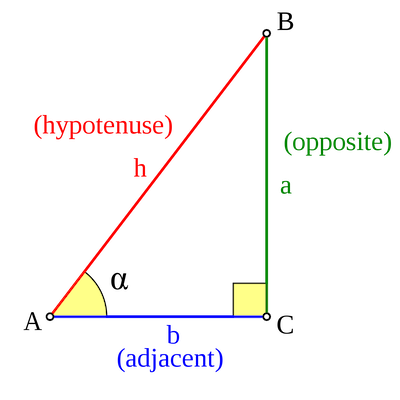
For the angle α, the sine gives the ratio of the length of the opposite side to the length of the hypotenuse. The cosine gives the ratio of the length of the adjacent side to the length of the hypotenuse. (Image by Dnu72 – CC BY-SA 3.0.)

The sine and the cosine functions can do a lot more than help you solve geometry problems. They can be used to build any waveform — the music you are listening to, the digital signal you are sending over wifi, even the swell on the sea — no matter how complicated these natural or human made oscillations might be.

Going round and round

The first step to constructing a wave is to imagine a circle of radius 1 drawn in Cartesian coordinates, with the centre of the circle lying at the point $(x,y)=(0,0).$ Imagine moving around the circle in an anticlockwise direction, starting at the right-most point, $(1,0)$. After you have rotated through an angle of $\alpha$ that is less than 90 degrees (corresponding to less than $\pi /2$ in radians) the point $(x,y)$ you are at defines a right-angled triangle, with corners $(0,0),(x,0)$ and $(x,y).$ The hypotenuse of this triangle has length 1 because the point $(x,y)$ lies on our circle of radius is 1. For this triangle we have $cos(\alpha )=x$ and $sin(\alpha )=y.$

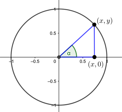
A right-angled triangle formed from a point on the unit circle.

You can continue to move around the circle anti-clockwise to make the angle $\alpha$ bigger than $\pi /2.$ When you do this, the triangle with corners $(0,0),(x,0)$ and $(x,y)$ no longer has $\alpha$ as one of its angles.

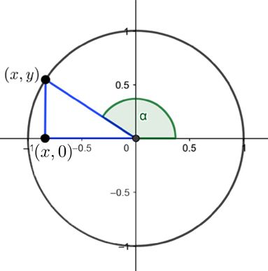
When α is greater than π/2, then the right-angled triangle formed from a point on the unit circle no longer contains the angle α.

However, there is nothing to stop you from extending the definitions of the sine and cosine of $\alpha$ in analogy with what we had before: $$\cos (\alpha )=x\text{and}\sin (\alpha )=y,$$ where $(x,y)$ are the coordinates of the point you are at.

What happens to the sine and cosine as you move once around the circle? In one circuit of the circle you will have turned through an angle of $2\pi$. As you moved around the circle your vertical coordinate (the sine) started at $0$ and increased steadily until it reached a maximum of $1$ when you were on top of the circle. As you kept moving it then dropped down to $0$ again in a symmetrical fashion, before reaching a minimum of $-1$, and finally coming back up again to 0.

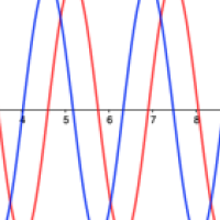
If you plot how the vertical coordinate (in red in the figure below) varies with the angle turned through (from 0 to $2\pi$) you get a regular wave shape. It starts at 0, goes up to the maximum of 1, then down to 0 again, before dropping to the minimum of -1, and up again to 0.

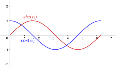
The red wave is the sine of the angle plotted against the angle (coming from the vertical coordinate) and the blue wave is the cosine of the angle plotted against the angle (coming from the horizontal coordinate).

This wave pattern repeats as you carry on going around your circle a second time, increasing the angle you turned through from $2\pi$ to $4\pi ,$ and a third time travelling from $4\pi$ to $6\pi$, and so on. You end up with an infinitely long, perfectly regular wave. The horizontal coordinates (the cosine) give a similarly perfect wave (plotted in blue above), offset against the first one by a distance of $\pi /2$ along the horizontal axis. This extends our definition of the sine and cosine to angles greater than $\pi /2$. (You can also define the sine and cosine for negative numbers by going round the circle in a clockwise direction.)

The red wave is the sine of the angle plotted against the angle (coming from the vertical coordinate) and the blue wave is the cosine of the angle plotted against the angle (coming from the horizontal coordinate).

Squeezing and stretching

We've now seen how moving around the unit circle can give us two functions, the sine function and the cosine function, each of which comes with a graph that describes a regular wave. When you encounter these functions in text books the variable is usually called $x$ rather than $\alpha$, so you will see something like $$f(x)=\sin (x)\text{and}g(x)=cos(x).$$ We will switch to this notation now. This means that $x$ now represents what used to be our angle $\alpha$ and that it no longer represents a coordinate of a point on the unit circle. That's potentially a little confusing, but hang in there and you will get used to it.

The wavelength is the distance between two peaks of a wave, and in our example so far this is $2\pi$. That's because to go through one complete cycle of our wave we had to turn through an angle of $2\pi$.

It's also possible to create waves with different wavelengths. To create a wave with wavelength $\lambda$ you multiply the variable $x$ by $2\pi /\lambda$ to get the functions $$f(x)=\sin \left(\frac{2\pi }{\lambda }x\right)\text{and}g(x)=\cos \left(\frac{2\pi }{\lambda }x\right).$$ By making the wavelength shorter you essentially squeeze the wave and by making it longer you stretch it.

In the Geogebra applet below, use the slider to change the wavelength of the sine (red) and cosine (blue) waves.

Going higher and going lower

The peaks of the waves we have created so far have the value 1 and the troughs have the value -1. To create a wave that has higher peaks and lower troughs, you simply multiply the entire function by a constant $A$ to get $$f(x)=A\sin \left(\frac{2\pi }{\lambda }x\right)\text{and}g(x)=A\cos \left(\frac{2\pi }{\lambda }x\right).$$ This constant is called the amplitude of the wave}.

In the Geogebra applet below use the sliders to vary the amplitude $A$ and wavelength $\lambda$ for the sine wave (red) and the cosine wave (blue).

Speeding up and slowing down

So far the waves we have created are stationary: they don't change over time. However, it is also possible to create waves that travel along. Our wave function will now be a function of two variables $x$ and $t.$ As before $x$ represents the position on the horizontal axis, while $t$ denotes time. Suppose you want your wave to be moving along at a speed of $v.$ The functions $$f(x,t)=A\sin (\frac{2\pi }{\lambda }x-vt)\text{and}g(x,t)=A\cos (\frac{2\pi }{\lambda }x-vt).$$ produce such moving waves. If you are keeping the time variable $t$ fixed then you are essentially seeing a snapshot in time, giving you a stationary wave just like the ones we had above. If you are keeping your location $x$ on the $x$-axis fixed, then you are seeing the corresponding $y$-variable as it moves up and down over time. This is a bit like watching a particular point on the surface of a lake move up and down as waves ripple through.

In the Geogebra applet below use the slider to change the speed. Setting the speed to 0 (or pressing the pause button) corresponds to stopping time, so you're keeping the time variable $t$ fixed. In this case you see a snapshot in time which looks like and ordinary sine (or cosine) wave, only perhaps shifted along the horizontal axis by some distance. Focusing on the blue dot corresponds to keeping the variable $x$ fixed. (We are not giving you the option of changing the wavelength and amplitude here as too much choice can be confusing!)

The reason the argument of our functions now is $x-vt$ is that in a time period of length $t$ a wave travelling at speed $v$ will have travelled a distance of $vt.$ The height of the wave at point $x$ along the $x$-axis at time $t$ will therefore be the same as the height was at time 0 at the point $x-vt,$ because that's how far the wave has travelled in time $t$.

Decoding messages

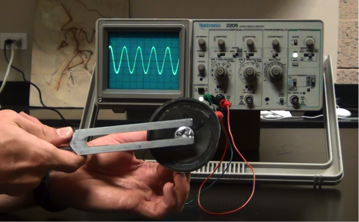
At first sight these sine and cosine waves we have created appear too perfect to tell you much about the waves we encounter in real life. But you can hear one in action if you strike a tuning fork. The sound you hear is the result of the vibrations of your ear drum, stimulated by the sound wave from the tuning fork travelling through the air. For a tuning fork, if you plotted the intensity, or pressure, of this vibration over time, you would see a perfect sine wave in action.

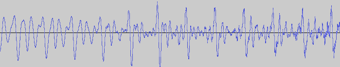
The sound wave from a tuning fork (top), compared with that of human speech (bottom).

As you can see the sound wave of something like speech is more complicated. But any sound wave, indeed any repeating function, can be broken up into a number of sine waves of various frequencies and amplitudes (intensities). This is the result of work that started with the French mathematician Joseph Fourier, who lived through the French revolution in the eighteenth century. The expression of a sound wave, or any signal varying over time, as the sum of its constituent sine waves, is known as the Fourier transform of that signal. (You can read a more detailed explanation of the maths involved here — the maths is quite complicated but the mathematical ideas involved are lovely!)

The function f varies in time – representing a sound wave. The Fourier transform process takes f and decomposes it into its constituent sine waves, with particular frequencies and amplitudes. The Fourier transform is represented as spikes in the frequency domain, the height of the spike showing the amplitude of the wave of that frequency.

About this article

This article was produced as part of our coverage of the Dispersive hydrodynamics: mathematics, simulation and experiments, with applications in nonlinear waves programme hosted by the Isaac Newton Institute for Mathematical Sciences. You can find more content about the programme here.

Rachel Thomas and Marianne Freiberger are the Editors of Plus.

This article is based on the book Numericon: A journey through the hidden lives of numbers by Marianne Freiberger and Rachel Thomas and our article Fourier transforms of images.

This article was produced as part of our collaboration with the Isaac Newton Institute for Mathematical Sciences (INI) – you can find all the content from the collaboration here.

The INI is an international research centre and our neighbour here on the University of Cambridge's maths campus. It attracts leading mathematical scientists from all over the world, and is open to all. Visit www.newton.ac.uk to find out more.