The concept of a tree of life was popularised by Charles Darwin through his theory of evolution through natural selection. The idea is that all species evolved from a common ancestor. Evolution means that at certain points in time a species might split into two new species, which then continue to evolve on their own, perhaps splitting again at some point in the future. When you draw a picture of this you do indeed get something looking a bit like a tree (upside down in the picture below), with today's species at the ends of the branches. The problem is that given a number of species, there is more than one tree that potentially describes their relationships. For example, given three species, there are three potential trees:

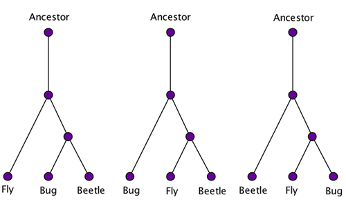
There are three different trees describing the possible genetic relationships between three species.

So here’s a question: given species, how many different possible trees of life are there?

We can answer this by doing a bit of counting. First of all, let’s be clear about what kind of object we are counting. We’ll assume that a tree of life looks something like the picture below. There is a root which represents the common ancestor. We assume that species can split into at most two (not three or more) other species at a time. Such trees are essentially what mathematicians call rooted binary trees. The tips of the branches, which represent the species alive today, are called the leaves of the tree. A line segment in the tree that connects two neighbouring branching points, or a branching point and a leaf, is called an edge.

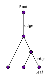
This is a rooted binary tree. (Strictly speaking, a rooted binary tree has two edges attached to the root, rather than one, but that distinction is not really important here.)

It’s not too hard to convince yourself that a rooted binary tree with leaves has a total of edges. You can do this by playing around with a few of these trees, or, much better, by using a proof by induction. A binary rooted tree with leaves obviously has edges. And since equals for this fits the bill.

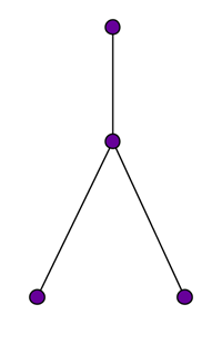
A rooted binary tree with two leaves has three edges.

Now suppose the claim holds for any rooted binary tree with leaves. That is, any rooted binary tree with leaves has edges. Now any rooted binary tree with leaves can be created from one with leaves by picking an existing edge, dividing it in half by a new branch point and have the new leaf sitting on the end of a new edge emanating from the new branch point.

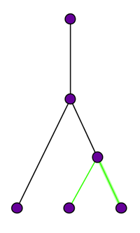
Here a rooted binary tree with three leaves has been created from one with two leaves by dividing an edge into two (a green and a black segment) and attaching the leaf to the end of an edge (green) that emanates from the new branch point.

This procedure creates two new edges that weren’t there before. So if, by our induction assumption, the tree with leaves had edges, then the tree with leaves has edges. This proves the fact that any rooted binary tree with leaves has edges.

How does that help us count the number of trees with leaves? Well, first of all notice that if is the number of trees with leaves, then the number of trees with leaves is That’s because, as we have already seen above, a tree with leaves can be made from one with leaves by attaching the new leaf to one of the existing edges. So for every rooted binary tree with leaves there are rooted binary trees with leaves: one for every edge of the first tree.

But what is the number of rooted binary trees with leaves? Well, we can make a rooted binary tree with leaves out of one with leaves, just as we made a tree with leaves out of one with leaves. Now, a rooted binary tree with leaves has fewer edges than a rooted binary tree with leaves. Since a new leaf is attached to one of the edges, we can therefore make two fewer trees with leaves out of trees with leaves than we can make trees with leaves out of trees with leaves. Writing for the number of trees with leaves, there therefore are

trees with leaves.

Similarly, writing for the number of trees with leaves, we see that

You might be able to see where this is going. Working your way backwards, the number of trees with leaves is

This expression is often written as the double factorial

It grows very quickly with For there are

rooted binary trees.

For there are rooted binary trees. And for there are rooted binary trees. That’s one of the problems facing people who study evolution. Even for a small number of species there is a huge number of potential trees describing their potential relationships.

You can read more about the maths of trees of life in Reconstructing the tree of life and Evolution: It's as real as gravity.

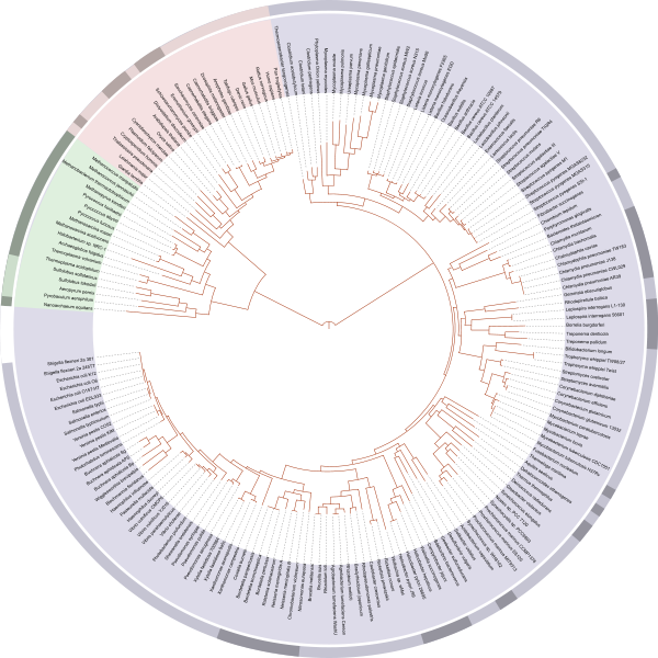
A tree of life, showing the relationship between species whose genomes had been sequenced as of 2006. The very centre represents the last universal ancestor of all life on earth. The different colors represent the three domains of life: pink represents eukaryota (animals, plants and fungi); blue represents bacteria; and green represents archaea. Note the presence of homo sapiens (humans) second from the rightmost edge of the pink segment. Click here to see a larger version of this picture.