Saving lives: the mathematics of tomography
Back to the Do you know what's good for you package
Back to the Constructing our lives package
Can Maths really save your life? Of course it can!! Maths has applications to many problems that are vital to human health and happiness. In this article we are going to describe how the mathematics of tomography has become one of the most important applications of mathematics to the problems of keeping you alive. Modern medicine relies heavily on imaging methods, starting with the early use of X-rays at the start of the 20th century.
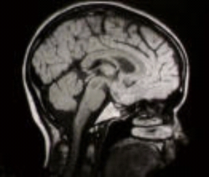
A CAT scan of the inside of a head.
Essentially these imaging methods take two forms. X-ray and ultrasound methods use a source of radiation that lies outside the body. The radiation is detected after it has passed through the body, and an image constructed from the way it has been absorbed. When X-rays are used, this process is called computerised axial tomography or CAT for short. (The word tomography comes from the Greek work tomos meaning "cut" or "slice".) This article will look at this process in detail.
Other imaging methods use a source inside the body. These include magnetic resonance imaging (MRI), positron emission tomography (PET) and single photon emission computed tomography (SPECT). These methods have certain advantages over CAT, both in image resolution and in safety, as X-rays can easily damage soft tissue. The basic mathematics behind tomography was worked out by the mathematician Johann Radon in 1917. Much later, in the 1960s Allan McLeod Cormack, working in collaboration with Godfrey Newbold Hounsfield, developed the first practical scanning device, the celebrated EMI scanner. For this work, Cormack won the Noble Prize. Early models could only scan an object the size of a human head, but whole body scanners followed shortly after.
Medical imaging works because of a combination of very careful measurement techniques, sophisticated computer algorithms, and powerful mathematics. It is the mathematics that we will describe here. We will also show that the mathematics of tomography has many other applications, including imaging the atmosphere, detecting land-mines and, slightly more frivolously, solving Sudoku puzzles.
Milk deliveries and Killer Sudoku
Before delving into the depths of medical science, we will start with a simple example which illustrates the principles of tomography, and which has a very nice link to the various types of Sudoku that have become very popular recently. This example involves milk deliveries. Imagine that milk and fruit juice is delivered in bottles that are placed in trays with 9 compartments arranged as a 3 × 3 grid. Each compartment of the tray contains a bottle which may contain milk, juice or be empty. The question is: which type of bottle is in which compartment?
Unfortunately, other trays are above and beneath the one we're interested in, so we can't look down on top of the tray. At first sight it would seem impossible to solve this problem. However, we can peer in through the sides and we can measure how much light is absorbed in different directions. Different types of bottle absorb different amounts of light. Careful measurements have shown that milk bottles absorb 3 units, juice bottles 2 units and empty bottles one unit. If a light beam is shone through several bottles, then this absorption adds up. If, for example, a light beam shines through a milk bottle and then a juice bottle, then 5 units are absorbed. If it passes through three empty bottles then 3 units are absorbed.
In the example below we have indicated the total amount of light absorbed when shining light through each of the rows and each of the columns.
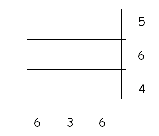
To solve this puzzle, we must place a bottle with 1,2 or 3 units of light absorption in each compartment, with the sum of the units in the first row equalling 5, in the second row 6 etc. The middle column contains 3 bottles and also absorbs 3 units of light. The only way this can be done is for each compartment of the middle column to contain one empty bottle absorbing one unit of light each. What about the other compartments? Unfortunately we don't have enough information (yet) to solve this puzzle. Here are two different solutions:
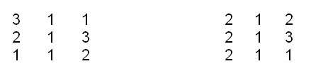
We are faced with a rather unusual situation for a mathematician in that we have two perfectly plausible solutions to the same problem. Problems like this are called ill-posed and are common in situations where we are trying to extract information from an image. To find out exactly how the bottles are distributed, we need to put in a little extra information. One obvious extra thing we can measure is the light absorbed in the two diagonals of the tray. We do this and find that 6 units are absorbed in the top left to bottom right diagonal, and 3 units in the bottom left to top right diagonal. From this extra piece of information it is clear that the first solution, and not the second, corresponds to the measurements made. It can be shown with a bit of extra maths, that if we can measure the light absorbed in the rows, columns and diagonals exactly, then we can uniquely determine the arrangement of the bottles in the compartments of the tray.
This problem may seem trivial, but it is very similar to the medical imaging problem we will describe in the next section, and shows how important it is to obtain enough information about a situation to make sure that we know what is going on exactly.
If any of this looks familiar to newspaper readers, then it is. Killer Sudoku is an advanced version of the popular Sudoku puzzle. In Killer Sudoku, as in Sudoku, the player is asked to place the numbers 1 to 9 in a grid with each number occurring once and once only in each row and column. However, rather than giving the player some starting numbers (as in Sudoku) Killer Sudoku tells you how the numbers add up in certain combinations. This is precisely the same as the problem described above.
CAT and the Radon Transform
Until relatively recently, if you had something wrong with your insides, you had to be operated on to find out what it was. Any such operation carried a significant risk, especially in the case of problems with the brain. However, this is no longer the case; as we described in the introduction, doctors are able to use a whole variety of scanning techniques to look inside you in a completely safe say. A modern Computerised Axial Tomography (CAT) scanner is illustrated on the left.
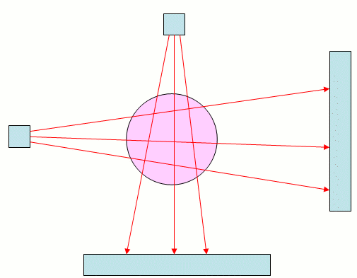
In this scanner the patient lies on a bed and passes through the hole in the middle of the device. This hole contains an X-ray source which rotates around the patient. The X-rays from this source pass through the patient and are detected on the other side. The level of intensity of the X-ray can be measured accurately and the results processed. The resulting fan of X-rays is illustrated in the following figure (with a conveniently circular patient).
As an X-ray passes through a patient, it is attenuated so that its intensity is reduced. The degree to which this happens depends upon what material the ray passes through: its intensity is reduced more when passing through bone than when passing through muscle, an internal organ, or a tumour. A key step in reconstructing an image of the body from a set of X-ray measurements is to carefully measure exactly how different materials absorb X-rays.
When an X-ray passes through a body, it does so in a straight line, and its total absorption is a combination of the amounts to which it is absorbed by the different materials that it passes through. To see how this happens, we need to use a little calculus. Imagine that the X-ray moves along a straight line and that at a distance $s$ into the body it has an intensity $I(s)$. As $s$ increases, so $I(s)$ decreases as the X-ray is absorbed. Now, if the X-ray travels a small distance $\delta s,$ its intensity is reduced by a small amount $\delta I$ . This reduction depends both on the intensity of the X-ray and the optical density $u(s)$ of the material. Provided that the distance travelled is small enough, the reduction in intensity is related to the optical density by the formula $$\delta I = -u(s)I(s)\delta s.$$ Now, when the X-ray enters the body it will have intensity $I_{start}$ and when it leaves it will have intensity $I_{finish}$. We can combine all of the contributions to the reduction in the intensity of the X-ray given by all of the parts of the body that it travels through. Doing this, we find that the attenuation (the reduction in the intensity) is given by $$I_{finish} = I_{start} e^{-R},$$ where $$R = \int u(s) ds.$$ This is the attenuation of one X-ray and it gives some information about the body. Below we see an object irradiated by several X-rays with the intensity of the rays measured on a detector. Here some X-rays pass through all of the object and are strongly absorbed so that their intensity (recorded at the centre of the detector) is low, while others pass through less of the object and are less strongly absorbed. Effectively the object casts a shadow of the X-rays and from this we can work out its basic dimensions. We illustrate this below.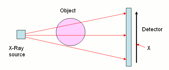
The intensity of the X-ray where it hits the detector depends on the width of object and the length of the path travelled both through the object and the air.
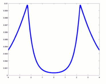
This graph shows the intensity of the rays as they hit the detector. Rays that travel through the full width of the object have lowest intensity, as we can see from the dip in the middle of the graph. Rays that just miss the body have the highest intensity, because of all rays that are not absorbed they travel the shortest distance. This is reflected by the two spikes of the graph. Towards the edges the graph falls off, reflecting the fact that the corresponding rays have travelled a comparatively long distance.
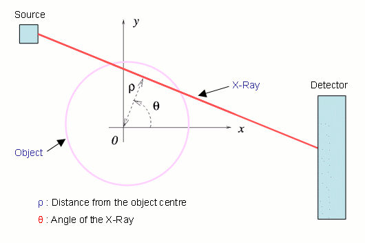
Incidentally, this is exactly the same problem faced by our milk deliverer in the previous section. The short answer to this question is YES, provided that we can make enough accurate measurements. A complete explanation of this, together with a quick way of calculating $R(\rho, \theta)$, is given in this section (for the brave). However, a quick motivation will be given by the following example. In the two figures below we see on the left a square and on the right its Radon transform in which the large values of $R(\rho, \theta)$ are shown as darker points.
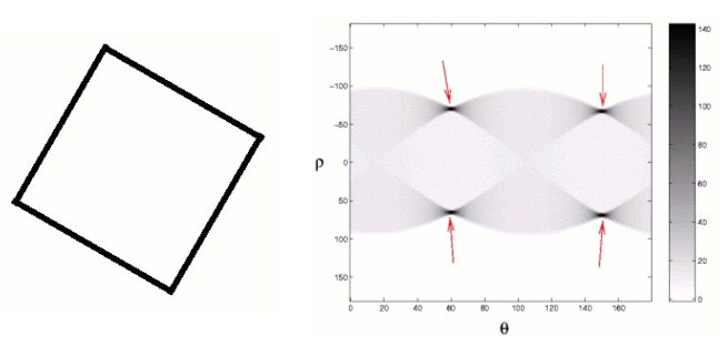
Basically the Radon transform is good at finding straight lines in an image. One method for finding $u(x,y)$, called the filtered back projection algorithm, works (roughly) by assuming that the original image is made up of straight lines and drawing those corresponding to the high values of $R$. This method is fast but not particularly accurate. However, it is possible to find $u(x,y)$ accurately and quickly, and algorithms to do this are implemented in the scanning devices. The original development of such devices uses a mathematical object known as Fourier transform to invert Radon transforms. If you're up for some serious maths, read the section on how this is done. Most of the maths here is university level, but the section contains some lovely mathematical ideas.
Tomography has many applications quite different from those in medicine. An interesting example comes from archaeology, where tomography was used to determine the cause of Tutankhamen's death. A CAT scan of the mummy revealed a swelling in the knee, indicating that death was the result of a massive infection. The cause of this was probably an injury inflicted by a fall. Whether Tutankhamen was pushed or fell by accident, however, will have to remain a mystery which even a CAT scanner cannot solve.
More generally, we can apply tomography to any problem where we have information about the average of a function along a straight line. It can also be used to find evidence for straight lines in an image (such as the edge of an object). We will now describe two examples of how tomography is used.
Tomography, GPS and how to land an aircraft safely
Orbiting the Earth are a large number of GPS satellites that are transmitting radio signals down to the ground. If you can detect the signals and find the phase difference between the signals from several different satellites, then you can work out your location with a high degree of accuracy. GPS positioning methods are very widely used by aircraft navigation systems, SATNAV devices and hikers. However, one of the problems with this system is that variations in the ionosphere (the upper part of the Earth's atmosphere) can affect the radio signals and change their phase by small amounts. This phase change can lead to errors in the position given by the GPS system. These are not very large and are perfectly acceptable for navigating. However, when landing an aeroplane it is vital that its height is known to very high precision and even small GPS errors can have large consequences. Here an accurate understanding of the state of the ionosphere is essential.
There are many other reasons why understanding the ionosphere is important. Chief amongst these is that fact that the ionosphere has a very significant effect on the propagation of radio waves and on communication in general. Roughly speaking, radio waves can bounce off the ionosphere, greatly increasing the range of a radio transmitter.
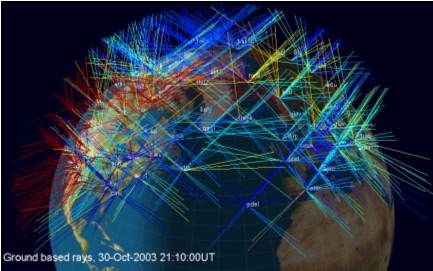
Remarkably, it is possible to monitor the state of the ionosphere using tomography. In the problem of imaging a patient we shone X-rays through their body. To image the ionosphere we use the transmissions from the GPS satellites. These form a very convenient set of "straight lines" passing through the ionosphere. The paths that they take are shown in the figure below.
The phase of the radio waves is affected by the electron content of the atmosphere, so that the total change in the phase is proportional to the integral of the electron density along the ray path. If we can measure these phase changes, then we can estimate the electron density integrals and work out the Radon transform of the electron density. We seem to be in exactly the same situation as in the medical imaging problem and hence able to work out the electron density at any point in the atmosphere.
Well, not quite. There are two big differences between this problem and the CAT problem. Firstly, the satellites are usually moving relative to the Earth. Secondly, there are large parts of the Earth's surface where we cannot make any measurements. These include the oceans, where there are no receivers for the satellite signals, and the poles, which do not have satellites orbiting above them. Thus we have a lot less information than we had in the case of the CAT scanner. This means that we are often in the situation of the milk deliverer who couldn't distinguish between two different arrangements of milk bottles, each of which led to the same set of measurements.
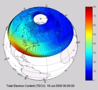
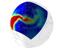
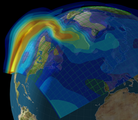
To get round this problem in the case of the ionosphere, we have to use a-priori information about the state of the ionosphere, or in other words a reasoned guess of what the solution should look like. This will allow us to reject one solution which doesn't look like this guess and to choose the solution which looks as much like the guess as possible. Fortunately, we understand the physics of the ionosphere well enough for our reasoned guess to be pretty close to the truth. By doing this (together with some other clever refinements) it is possible to use tomography to find the state of the ionosphere. In the figures below we illustrate a calculation (using the MIDAS software developed at the University of Bath) of an ionospheric storm (in red) developing over the southern part of the USA.
 |
 |
 |
Detecting land-mines
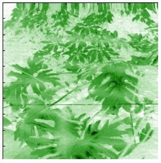
Can you find the three trip-wires hidden in this image?
Anti-personnel land-mines are one of the nastiest aspects of the modern warfare. They are typically triggered by almost invisible trip-wires attached to the detonators. Any algorithm for the detection of trip-wires must work quickly and not get confused by the leaves and foliage that obscure the wire. An example of the problem that such an algorithm has to face is given in the figure below, in which some trip-wires are hidden in an artificial jungle.
Finding trip-wires involves finding partly obscured straight lines in an image. Fortunately, just such a method exists; it is the Radon transform! For the problem of finding the trip-wires we don't need to find the inverse, instead we can apply the Radon transform directly to the image. Of course life isn't quite as simple as this for real images of trip-wires, and some extra work has to be done to detect them. In order to apply the Radon transform the image must first be pre-processed to enhance any edges. Following the application of the transform to the enhanced image a threshold must then be applied to the resulting values to distinguish between true straight lines caused by trip-wires (corresponding to large values of R) and false lines caused by short leaf stems (for which R is not quite as large).
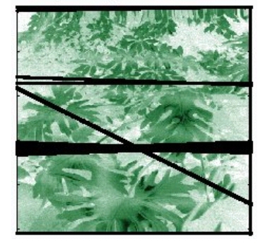
Following a sequence of calibration calculations and analytical estimates with a number of different images, it is possible to derive a fast algorithm which detects the trip-wires by first filtering the image, then applying the Radon transform, then applying a threshold and then applying the inverse Radon transform. The result of applying this method to the previous image is given on the left, with the three detected trip-wires are highlighted.
Note how the method has not only detected the trip-wires, but, from the width of the lines, an indication is given of the reliability of the calculation.
Maths truly does save lives!
You might also want to listen to our podcast on the Fourier transform.
About the authors
Chris Budd is Professor of Applied Mathematics at the University of Bath, and Chair of Mathematics for the Royal Institution. He is particularly interested in applying mathematics to the real world and promoting the public understanding of mathematics.
He has recently co-written the popular mathematics book Mathematics Galore!, published by Oxford University Press, with C. Sangwin.

Cathryn Mitchell is Professor of Electronic and Electrical Engineering and EPSRC Research Fellow at the University of Bath. She is interested in all sorts of tomography problems ranging from medical imaging to space physics.
This article now forms part of our collaboration with the Isaac Newton Institute for Mathematical Sciences (INI) – you can find all the content from the collaboration here.
The INI is an international research centre and our neighbour here on the University of Cambridge's maths campus. It attracts leading mathematical scientists from all over the world, and is open to all. Visit www.newton.ac.uk to find out more.
Comments
Anonymous
Many thanks for a beautifully accessible explanation of how tomography works!
Marrakesh architect
Anonymous
Thanks for your clear information; I think that your students are very lucky!
Best Regards.
M.Celaleddin Çetin
ITU foreign Languages School
Istanbul/Turkey
Anonymous
Having read Professor Stewart's excellent Cabinet of Curiosities, I was keen to read more about Radon Transforms and their applications which which this article achieves admirably. Thank you! Malcolm Golland, Potters Bar, England
PS Read while listening to a radio broadcast of an excellent performance of Bach's B Minor Mass from London's Royal Albert Hall. What a combination - my two passions in life viz. Mathematics and Music - marvellous!
Anonymous
I really liked the article. I'm trying to learn more about the fundamentals of this kind of equipment after medical school. The image at the beginning is a sagittal T1 weighted MRI (rather than a CT that is gathered axially). You can tell because the fat is high signal and bone is low whereas CT would have bright bone and less contrast within the brain.
The links were also especially helpful. Thanks for writing this.
Anonymous
Thank you so much for this clear information. I wish all professors would be able to explain like you are.
Anonymous
Hounsfield also won the Noble Prize. And although he used McCormack's work I don't think they collaborated on the scanner. The head photo is a CT Scan, a sagital view of axial images reformatted on the computer. You could not get your head sideways in the scanner
Maria
Great info! Landmine stuff was fascinating. But the second sentence of the second paragraph has a glaring error this x-ray student found: ultrasound does not use radiation, I think you meant CT!! :)