The growth rate of a disease

The growth rate of a disease is a natural way to capture how quickly the number of new infections are changing day by day. The growth of cases of a disease is modelled using an exponential curve:

$N(t) = {\rm constant} \times e^{\lambda t}$

Here $N$ is the number of cases, which depends on time $t$ measured in days, and $\lambda$ (pronounced "lambda") is what is called the growth rate of the disease per day. (The number $e$ is a mathematical constant approximately equal to 2.719 and intimately connected to exponential growth.)

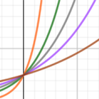
For example, the growth rate for HIV is $\lambda$ =0.002 per day and for measles is $\lambda$ =0.06 per day. You can use the interactivity below to explore how the progression of a diseases changes for different growth rates (use the slider to change the value of $\lambda$ ).

Back to the Epidemiology for beginners collection.

If the growth rate is positive, the number of new cases each day is increasing. And if the growth rate is 0, the number of new cases stays constant. What is needed to keep an epidemic under control is for the growth rate to be negative and hence the number of new cases to be decreasing.

But what does the value of the number actually mean? If the number of new cases has decreased by 3% since yesterday, then the growth rate is, approximately, $\lambda$ = -0.03 per day. (This isn't exactly equivalent but a good approximation for typical values of $\lambda$ . The growth rate actually works like compound interest which you can read about here.) Conversely, for small values of $\lambda$ (eg $\lambda =0.01$ ), the value of lambda approximates the percentage growth in cases per day: $\lambda =0.01$ means that cases will increase by around 1% a day.

However, for larger values of lambda (eg $\lambda =0.35$ ) this approximation is no longer accurate. In this case the percentage growth from one day to the next is $e^\lambda -1$ : for example for $\lambda =0.35$ that's $0.42$ ). (For a more detailed explanation of the relationship between the growth rate and the percentage growth per day read The doubling time of a disease.)

Why isn't R enough?

If you have already studied a bit of epidemiology, you have probably come across the concept of R, the reproduction ratio (or sometimes called the reproduction number) of a disease. That's the number of people infected, on average, by a single infected person. As explained here, R helps us understand what is happening with the disease: R>1 means that the epidemic will grow, R=1 means we are plateauing, R<1 means that the epidemic will decline.

One thing that R does not tell us, though, is how quickly things are changing. This is because R is not a rate, there is no timescale involved. For example, if R=2 for some disease then we know the epidemic will grow (because R>1), but we cannot tell how quickly. For diseases like HIV or TB, where there can be months or years between one person infecting the next person, even R=2 means slow growth over time. However for influenza or measles, where the infection is much faster, on the scale of days, R=2 means very rapid growth.

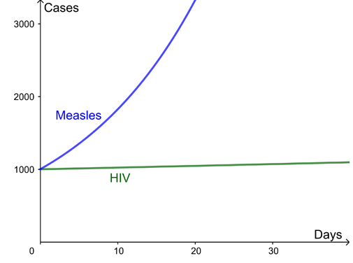
Here are two example curves for the growth of infection, both with a reproduction ratio R=2. The difference is the time between new infections – several months for HIV but just days for measles.

Which is better: R or the growth rate?

Both the reproduction ratio $R$ , and the growth rate, $\lambda$ , are valid measures for understanding the growth of a disease. They each have their uses, as outlined below:


Reproduction ratio: R	Growth rate per day: $\lambda$
R is more natural for understanding strength of the intervention needed to stop an epidemic, better for planning control measures. For example: R=1.5 means we need to reduce transmission by one third. R=2 means need to vaccinate half the susceptible people (you can read about this calculation here); R thus gives an intuitive way of predicting the strength of future interventions needed to stop an epidemic.	Growth rate is more natural for thinking about how cases change over time. For example $\lambda = 0.01$ per day means cases will increase by about 1% a day. $\lambda = -0.02$ per day means cases will decrease by about 2% a day. The growth rate is a good description of what's happening now: if we have a certain number of cases today then we can work out how many to expect tomorrow, the day after, and so on.
R>1 exponential growth R=1 flat R<1 exponential decay	$\lambda >0$ exponential growth $\lambda = 0$ flat $\lambda <0$ exponential decay
R a ratio of cases by infection generation. It is not a rate: there is no timescale involved.	The growth rate $\lambda$ is a rate.
R is not at all easy to measure in practice, but can be fitted using models if the timescales of infection are known. In principle it could be estimated by detailed epidemiological data on exactly who got infection from whom, but this is not usually feasible in typical settings.	The growth rate $\lambda$ is relatively easy to estimate from time series data of cases or deaths (but see below about small numbers). A simple approach is just to find the gradient of the logged cases. More advanced approaches, which can take into account a time-varying growth rate, or heterogeneous population, again involve fitting epidemic models.

Both the reproduction ratio and the growth rate are particularly hard to estimate when the number of cases is small, for example if the incidence of the disease is very low, or if the community you are studying has a very small population. In that case, day to day fluctuations can easily swamp the underlying patterns of the disease, so you will have greater uncertainty about the growth rate (and so expect wider confidence intervals).

How do you get from R to the growth rate and vice versa?

The precise relationship between R and the growth rate is not straightforward: it needs to take into account the timings of each infection to the next. A crude approximation is

$R=e^{\lambda T},$

where $T$

is the mean generation time: the time from one infection to the next.

I can cope with some advanced maths, tell me more!

OK! All of this supposes that the control measures and number of people susceptible to the disease are not changing too quickly.

Following one infected person, denote their time since infection by $\tau$ (in days). They go on to infect $R$ others on average. For each of these, their timing of infection is distributed with probability density function $f(\tau )$ . Then (exercise for maths undergraduates!) $R$ and $\lambda$ are related as follows:

$R^{-1} = \int _{\tau =0}^{\infty } e^{-\lambda \tau } f({\tau }) d\tau$

and yes, this is very closely related to a Laplace transform, or a moment generating function for the generation time distribution.

For specific distributions for the generation time, for example a gamma distribution, this can sometimes be simplified. Taking the generation time to be exactly constant, say $T$ , we recover the $R = e^{\lambda T}$ , but this is a rather crude approximation for many infectious diseases in practice.

Note, $f(\tau )$ depends on a variety of things, including biological things like the incubation period, and on social factors like whether you still mix with others when you have symptoms or if you self-isolate.

See this paper by Wallinga and Lipsitch for more details.

About this article

Rachel Thomas and Marianne Freiberger are the Editors of Plus. This article was produced with Julia Gog, Professor of Mathematical Biology at the University of Cambridge and co-lead of the JUNIPER network. Gog is also a member of the Scientific Pandemic Infections group on Modelling (SPI-M), an advisory group of the Department of Health and Social Care which provides expert advice to the UK government based on infectious disease modelling and epidemiology and fed results into the Scientific Advisory Group for Emergencies (SAGE) during the COVID-19 pandemic.

This article is part of our collaboration with JUNIPER, the Joint UNIversities Pandemic and Epidemiological Research network. JUNIPER is a collaborative network of researchers from across the UK who work at the interface between mathematical modelling, infectious disease control and public health policy. You can see more content produced with JUNIPER here.