Matrix: Simulating the world Part II: cellular automata

Welcome to a virtual world. Even complex processes can be modelled with relatively simple cellular automata.
In the first part of Simulating the World we saw how simple mathematical models can be built to study everything from the flocking of birds to the collision of entire galaxies. In these examples, a matrix, or a grid of numbers, was used as a convenient way of storing information on all the objects included in the simulation, so that it can be updated each time step as the simulation progresses. In this second article, we'll take a look at another class of mathematical models; ones where the matrix or array isn't just a way of storing information during the simulation, but actually is the simulation itself.
Many real-world situations can be simplified as a sequence of objects in a line or an arrangement across a flat space — in other words, they can be faithfully represented by either a list of numbers (a one-dimensional matrix) or a regular grid of cells (a two-dimensional matrix). During the course of the simulation, the objects interact with those near-by according to a set of predefined rules, with the identity of each discrete position on the line or plane changing over time. Such a system is called a cellular automaton model.
Cellular automata
The essence of any cellular automaton is a regular grid of cells, each of which can be in any one of a number of different states. The earliest cellular automata models used only two states and are said to be binary — each cell could be either ON or OFF. More complex models use a greater number of possible states, as we'll see a bit later on. Time is discrete, which means that at every time step the state of each cell is updated as if the cells were co-ordinated by the tick-tock of a great clock. The state of each cell is updated in accordance to a set of rules depending on the cell's current state and that of its neighbours. In a one-dimensional model, the neighbours are simply the cells to the immediate left and right of the one in question. In two dimensions there are different ways of defining the neighbourhood, but using the 8 bordering cells is one very common method.
Ideally, the simulation world would be infinite, with the grid of cells extending for ever in all directions, so that there is no concern about what to do with cells along the edge, which don't have the full number of neighbours. Handling this on a computer is obviously impossible in practice, and so the opposing world boundaries are joined into a circle (one-dimensional) or doughnut-shaped torus (two-dimensional), as we saw in the first article. This kind of model is said to have periodic boundary conditions.
One very famous example of a two-dimensional cellular automaton is the so-called Game of Life, where cells on the grid either die, survive, or are born, depending on the number of their neighbours already alive (ON). The rules for the universe are very simple, but even so, incredibly complex behaviour emerges out of the evolving patterns of cells. We won't go into the fun to be had with the Game of Life here though, as this is well covered elsewhere, and Plus has also interviewed its creator John Conway.
In this article, we'll take a look at examples of both one-dimensional and two-dimensional cellular automata, from traffic on a road to forest fires and cities.
Road traffic
In the very simplest road traffic set-up, we define the system so that each cell can exist in only two states. Here, 0 denotes that the cell is empty — clear road — and 1 denotes that the patch of road is occupied by a car. The neighbours of each cell are those immediately in front or behind. The scenario for this single-lane model is such that a car can only advance forward if the road cell to the right is clear, otherwise it stays put. We are only considering a single-lane road here — cars cannot overtake each other.
This model can be formally described as a set of rules for all eight (23) possible states of a cell and its two neighbours as follows (the change to the third cell obviously depends on the next one to the right, not shown):
1. 000 ⇒ 000
2. 001 ⇒ 000
3. 011 ⇒ 010
4. 010 ⇒ 001
5. 100 ⇒ 010
6. 101 ⇒ 010
7. 110 ⇒ 101
8. 111 ⇒ 110
Situation 1 is the simplest case; the cell in question, and both of its neighbours, are empty of cars and so nothing changes in the next time step. In numbers 2, 4, 5, and 7 one of the cars has clear road ahead, and so can advance one cell to the right, vacating the road space behind it. In situations 3 and 8, the central car finds another vehicle immediately in front of it, and so cannot move — there is a temporary deadlock in the road.
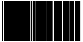
The display shows our strip of road as it changes over time. A vacant cell is represented by a black pixel and a cell with a car by a white pixel. There are no rules that cause the cells' states to change, so the traffic is stationary.
The evolution of this one-dimensional cellular automaton over time can be represented by displaying the sequence of changing strips of road one after the other down the page. So let's take the very simplest case, where the initial value in each cell is randomly assigned to either 1 or 0 (occupied by a car or empty), but where there are no rules defined for the evolution of the array from one time-step to the next. Let's take the probability of any cell containing a car at the beginning to be 1%. The image to the right shows the development of the cellular automaton as a simple series of vertical stripes — the value of each cell does not change over time (looking down the page) because all cars are stationary. Here black denotes an empty cell and white denotes an occupied cell.
Now that we understand what the lay-out of the display means, we can add in the rules (as above) so that a car can move forwards to the right if the road in front of it is clear. Now, the display becomes a little more complicated. The road is nice and empty of traffic, and so each car always finds the space immediately in front of it clear and so advances one cell to the right every time-step. One important aspect to remember about this cellular automaton is the periodic boundary condition: the road loops round into a complete circle, like the M25. So whenever a car drives off the right-hand side of the diagram, it reappears on the left-hand edge. This is shown well in the animation below. If you set the probability of a cell containing a car to 0.1 and click "start", you will see diagonal white stripes appearing. These represent cars driving steadily along the road, disappearing from the right-hand side and wrapping around to the left.
The cellular automaton gets a whole lot more surprising if we increase the number of cars on the road. Setting the probability of each cell containing a car during the initial set-up to be 50% — 0.5 in the animation — produces a different pattern. Many of the cars find the space in front of them empty and so advance one square to the right every time-step. Occasionally, the random assignation of a value to each square at the beginning places several empty cells next to each other, and these appear as thin black 45 degree diagonal stripes. These empty stripes are preserved over time because all the cars in this simple model are moving at the same speed, so they never catch up with those in front to close up the gaps in the traffic.
The white stripes are where cars have bunched up bumper-to-bumper on the road. Only the front car of this stationary clump can move away into empty road, while the stationary obstacle means that other cars have to stop at the back end, and so these traffic jams move steadily back up the road — appearing as a -45 degree white stripe.
Traffic nightmares? Modelling can not only imitate traffic flow, but also come up with traffic control mechanisms that can help alleviate congestion.
The most interesting behaviour shown by this extremely simple cellular automaton is when a right-moving black stripe intersects a left-moving white stripe. This is the situation when a gap in the flow of cars meets a temporary traffic jam. If the stripes are the same thickness (i.e. involve the same number of cars and car holes) they perfectly annihilate each other to result in a steadily-flowing stream of closely-spaced cars. Over time the number of black and white stripes inexorably decreases as they meet and cancel each other out, until only those which were slightly more frequent in the initial set-up survive.
Although this very simple cellular automaton already shows some interesting behaviour, it's easy to increase the complexity of the model to better represent traffic on a road. In reality, a stream of traffic on a road does not exist in one of only two states — stationary or moving forward at the same speed. There is in fact a smooth spectrum of different speeds that cars can take, as they accelerate over stretches of open road before getting caught behind slower-moving traffic ahead.
We can improve our cellular automaton model by allowing the cars to take different speed values. This is achieved by keeping a cell value of 0 to denote an empty road square, and assigning the values of 1 to 10 to denote a cell occupied by a car with that particular speed. If a car finds itself with a clear stretch of road in front it accelerates up to the speed limit (10 units per time step), otherwise it slows down to match the speed of the car just in front. In this case, the state of each cell in the one-dimensional array can be colour-coded: black still signifies a patch of empty road, with a cell containing a car moving at a speed of 1 - 10 denoted with a colour spectrum blue - red.
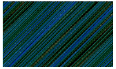
The display produced when speed is allowed to vary.
Besides producing a pretty multi-coloured striped pattern, this simple traffic flow model generates some startlingly realistic behaviour. As cars are constantly accelerating into empty road or braking behind slower-moving vehicles, the traffic spontaneously forms into packs of fast-moving cars and caravans of slow-moving cars. You can see this in the diagram as a series of orangey-red and greeny-blue stripes, respectively. The really interesting behaviour is when a train of fast traffic pulls up behind slower cars — the traffic is forced to slow and bunch up and then spaces out again as the cars accelerate away. This exactly reproduces the compression waves often seen in real traffic on road-layouts much more complicated than this simple scenario, with variable speed limits, multiple lanes and over-taking, and side streets feeding into main roads.
Two-dimensional cellular automata
When another dimension is added to the simulation, so that the cells are spread out across a plane, even more realistic simulations of natural phenomena can be created. A common two-dimensional cellular automaton model is that of fires spreading in a forest. Cells in the grid can contain only bare earth (grey cell), be occupied by trees (green cell), or by burning trees (orange cell). A grey cell becomes a green cell with a certain probability, simulating tree growth. A green cell that has no burning neighbour becomes red with a certain low probability. This simulates lightning strikes, or any other natural fire starter. Once ignited, a cell with a forest fire burns out in a single time-step, returning the cell to bare earth, but the inferno spreads to all adjoining cells filled with trees. The animation below allows you to set the probability of a tree cell igniting and the probability of an earth cell growing trees. Click "start" to see the scenario evolving. You can also see a full screen version.
The dynamics of our model forest mirror that of real woodland: trees grow slowly and spread into clear space, but are lost suddenly in catastrophes of small, medium and large fires. It turns out that the frequency distribution of fires follows a power-law: small fires strike regularly, medium-sized conflagrations occasionally, and great forest-spanning infernos happen only very rarely. This same pattern is seen in many natural events, from avalanches and earthquakes to meteorite impacts. Large fires become much more likely, though, if the sparking probability is low because the forest has time to grow up and thickly cover the land before being hit by the next wildfire.
Once again, a ludicrously simple model produces some very interesting behaviour. At any one time, depending on the assigned probability of fire-starting, several areas of forest will be burning simultaneously, in a range of small patches to large regions. If the forest has become particularly dense, large clusters of trees exist and isolated regions of forest fire can spread rapidly and merge together to cover larger and larger areas of the forest, before finally burning themselves out. The thicker the forest, the more devastating fires become, and the more land cover they consume and destroy. So even this simplistic model produces a somewhat counter-intuitive result: it may well be safer to allow regular small fires to burn naturally through a forested region than to always attempt to extinguish them as quickly as possible. Fire prevention officials are now actually deliberately starting small fires to prevent bigger, uncontrolled, infernos.
City development
Two-dimensional cellular automata models have not only been applied to understanding the natural environment, but also that of the human world. Sophisticated cellular automata models have been applied, for example, to studying the development of cities over time. The land area of a city is divided into cells, all of which have a certain neighbourhood of other adjoining cells, as before. But in this case you can allow the cells to take several different states simultaneously to reflect the great variety of combinations possible in a real city. For example, a small region of urban space can contain any of a number of different land uses (such as residential, retail, offices, industrial), at a range of densities (eg. from sub-urban bungalows to high-rise blocks on a housing estate), property values, and so on. Depending on the surrounding area, the identity of cells evolve over time, and the rules defining these transitions can themselves be very complex. And of course, the geography of the land itself can exert a strong influence on the development of a city, such as nearby hills, the course of a river, or the unconfining flat plains of a sprawling Los Angeles. One research group at Arizona State University is attempting to include all these sorts of factors into great simulations of future urban development. Imagine an automatic game of SimCity, but on a vast scale!
Further Reading:
- Cellular-automata models applied to natural hazards; Bruce Malamud and Donald Turcotte, Computing in Science and Engineering, Volume 2, issue 3, p.42-51 (May 2000).
- Computer code (Mathematica) used for simulating one-dimensional traffic flow.
About the author


Lewis Dartnell read Biological Sciences at Queen's College, Oxford. He is now on a four-year combined MRes-PhD program in Modelling Biological Complexity at University College London's Centre for multidisciplinary science, Centre for Mathematics & Physics in the Life Sciences and Experimental Biology (CoMPLEX). He is researching in the field of astrobiology — using computer models of the radiation levels on Mars to predict where life could possibly be surviving near the surface.
He has won four national communication prizes, including in the Daily Telegraph/BASF Young Science Writer Awards. His popular science book, Life in the Universe: A Beginner's Guide, has been reviewed in Plus. You can read more of Lewis' work at his website.
The animations in this article were produced by Ian Short. Ian is a post-doctoral researcher in mathematics in the National University of Ireland, Maynooth. He also works part-time for the Millennium Mathematics Project of which Plus is a part.