Births and deaths in fluid chaos
"Most of the Universe is filled with fluids of one kind or another," says Jerry Gollub, a Professor of Physics at Haverford College with a special interest in fluid dynamics. "They are important in astrophysics, they are important in engineering, in medicine and health, in chemistry, geophysics, basically in all the sciences. Fluid motion underlies natural phenomena both large and small, and there are many applications that affect society."
The Universe is filled with fluids.
People have long been fascinated by fluids. The ability of water to be so many different things — yielding but strong, embracing but free, serene, chaotic, or even angry — has inspired poets as well as scientists throughout history, and the scientific study of fluids can be traced back to Archimedes, and possibly further. Today scientists study all kinds of fluids, including gases, grainy fluids, sticky fluids and elastic ones. Applications range from the use of microfluids in nanotechnology, to understanding the flow of blood, the formation of tears in our eyes, aerodynamics, predicting weather patterns, or understanding the behaviour of gas clouds in outer space. Questions on the nature of fluid flow abound. "Fluid dynamics is not dominated by a few special questions in the way that, for example, the physics of elementary particles might be," says Gollub. "In fluid dynamics there is tremendous diversity."
But while much research in fluid dynamics is driven by applications, there are also fundamental questions that need to be answered. Even the most fundamental question of them all — how to best describe the flow of fluids mathematically — still hasn't been answered in full generality. It's all very well when a fluid flows smoothly down a channel, but how do you cope with the chaotic or even turbulent flow of, say, a raging mountain stream? It is in this area of chaotic flows that Gollub and his collaborator Nicholas Ouellette, now at Yale University, have made an interesting, possibly very significant, discovery, by combining experimental results with sophisticated mathematics.
Traditional approaches
To set the scene, let's first look at the traditional mathematical approach to fluid flow. Imagine you have a fluid moving around in a container and you want to describe its motion over a period of time. The most important descriptor of this motion is the velocity of the fluid at each point $(x,y,z)$ in space and at each point $t$ in time. Velocity is a vector; its direction indicates the direction of the fluid flow and its magnitude the fluid's speed. Since space and time are continuous, a full description would entail an infinite number of vectors, one for each location and instant. A function $v(x,y,z,t)$, which allocates a velocity vector to each point $(x,y,z)$ in space and instant $t$ in time is called a velocity field.
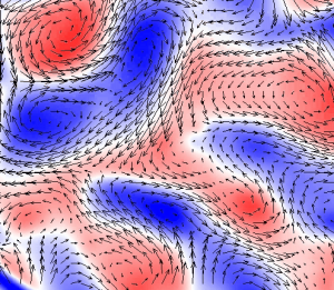
Figure 1: A snap-shot of a two-dimensional fluid with some of the velocity vectors shown. Blue and red indicate clockwise and counter-clockwise rotation. Fixed magnets and electric currents are used to drive the flow.
In some cases it is possible to derive the velocity field from the Navier-Stokes equations of fluid motion, which were established in the early nineteenth century by the physicists Claude-Louis Navier and George Gabriel Stokes. Their equations are based on the laws of conservation of mass and momentum, and relate the changes of velocity at different locations and instants. Since the equations involve rates of change, they are phrased in terms of derivatives, and are therefore known as partial differential equations. The solutions of this set of equations for given conditions, if you are able to find them, are precisely the possible functions $v(x,y,z,t)$.
This is the theory, but in practice things aren't that simple. Partial differential equations have a habit of being hard to solve, especially if they are nonlinear, and the Navier-Stokes equations are no exception. In some simple situations it is possible to obtain analytical solutions — solutions that can be written down explicitly — but in many physically interesting situations, for example in turbulent flows, analytical solutions are beyond reach. What's more, no-one knows if physically meaningful solutions even exist for the general case of a three-dimensional incompressible fluid. In fact, proving the existence or non-existence of general solutions to the Navier-Stokes equations is one of the most important open problems in mathematics; whoever solves it is set to win $1m from the Clay Mathematics Institute.
This might seem worrying seeing that so many products of modern engineering, including aeroplanes, are based on fluid dynamics. However, for practical purposes, scientists and engineers use theoretical methods, computer simulations or experimental data to approximate the velocity field at a large number of individual points in time and space. The numerical method works well, but requires an immense amount of computing power. "Suppose you wanted to describe the motion of fluid in a box that's 10cm across in each direction," says Gollub. "Maybe you'd like to know the velocity at spacings of 1mm. So on each axis you have to give 100 numbers. You have three axes, so altogether you have to specify 1 million numbers at each instant in time. You might be able to do this, but then what do you do with all that data? You'd really have great difficulty to test theoretical ideas, it's just too much information." The large number of variables can become difficult even for fast computers to deal with, and what's more, the brute-force numerical approach isn't exactly elegant. Surely there must be better ways of describing fluid flows?New ideas
Gollub believes in the power of experiment to reveal hidden patterns, and it was through experiment that he and Ouellette came up with their new discovery. Describing turbulence is something of a holy grail in fluid dynamics, and as a sort of precursor to turbulence, Ouellette and Gollub have addressed the problem of spatiotemporal chaos. Flows that exhibit spatiotemporal chaos are disorderly in space and also unpredictable in time, so that knowledge of the present state of the fluid will not make the next instant predictable. Instead, our ability to predict the future becomes progressively inaccurate as time passes. In fact, the uncertainty increases exponentially with time. This behaviour is complex, but not quite as wild as "strong turbulence", where motion on many scales (vortices of all sizes) occurs simultaneously. "We have been interested in studying flows that consist of a collection of vortices, or circulating areas," says Gollub. Such flows can exhibit spatiotemporal chaos. "How do you describe such a flow? Do you really need to use the full velocity field, as has been traditional, or can you get by with something simpler?"
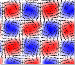
Figure 2: In this image, obtained experimentally by Ouellette and Gollub, the vortices form a regular array and do not fluctuate.
In their experiment Ouellette and Gollub considered a thin layer of a conducting fluid, where most of the fluid activity would occur in a horizontal plane. To track the flow, they released thousands of fluorescent polystyrene tracer particles into the fluid. They then set the fluid in motion using magnets and electric currents, which created a pattern of vortices. By changing the electric currents, they were able to control the complexity of the flow: for a small driving current, the vortices stay in fixed locations (see figure 2), while for a larger current, they break free and move around unpredictably. This latter scenario is a chaotic state. "Over time, the vortices arrange and rearrange themselves in an irregular way. The pattern looks different in ten seconds from what it looks like now, and it never seems to repeat itself." (Click on figure 3 to see a movie of this behaviour.)
Figure 3: Here the vortices have broken free from the regular lattice of driving forces, and evolve unpredictably in the state of spatiotemporal chaos.
Rather than describing this complex motion by measuring the velocity at a great number of points over time, Ouellette and Gollub decided to look for geometric features that characterise the whole flow. They were interested in two sets of special points: those that lie at the centre of vortices, known as elliptic points, and those towards which the flow converges along one direction, but from which it diverges along another direction. These are known as hyperbolic points, or saddle points (see figure 4). Elliptic points have the flow whirling around them, while hyperbolic points arise, for example, at a point where four vortices meet, with each neighbouring pair of vortices turning in different directions. These types of points tell you, at a given point in time, where vortices are centred, and where the domain of one vortex ends and another starts — very important information in a flow that is dominated by vortices. Could this information be enough to characterise the whole flow?
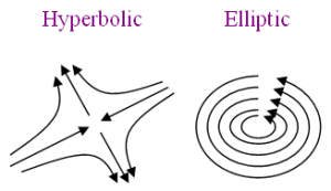
Figure 4: The flow of the fluid close to elliptic and hyperbolic points.
The idea was a good one, but there was a problem: how do you locate the special points? One possibility is to look for points of zero velocity, but this is hard to do accurately. But Ouellette had an ingenious idea. He noted that near elliptic points, tracer particles circulate in very small circles, and near hyperbolic points, they turn sharp corners. In both cases, the trajectories of particles exhibit very high curvature. Using ideas from differential geometry, Ouellette came up with a reliable way of locating the special points by measuring the curvature of the tracer particles' trajectories.
Creation and destruction
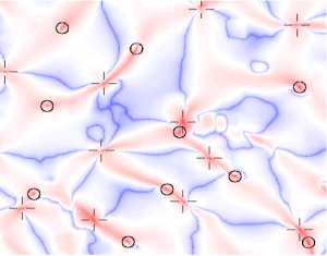
Figure 5: The fluid flow with the special points marked by circles (elliptic points) and crosses (hyperbolic points).
Once they had located the special points, Ouellette and Gollub tracked their behaviour over time, and found some amazing patterns. "The most interesting phenomenon is that the special points can be born, or die, always in pairs containing one of each type" Gollub explains. "You can have a hyperbolic and an elliptic point that annihilate each other, leaving no special feature in that region. You can also have the opposite, where a hyperbolic and an elliptic point are born together. It's very striking." (Click on figure 5 to see a movie of this behaviour.)
Striking it may be, but does it tell us anything useful about the system? Ouellette and Gollub forced the system using varying driving currents and measured the frequency of births and deaths for each forcing strength. They found an interesting correlation: "The rate at which births and deaths occur turns out to be an excellent measure of the strength of the chaos in the flow," says Gollub. The typical speed of a flow can be measured by a quantity called the Reynolds number (see Plus article The Buzz of the bumblebees for more information), and Ouellette and Gollub found that the rate of births and deaths rate grows linearly with the Reynolds number once a critical value is passed. "Furthermore, the rate correlates well with other measures of the strength of spatiotemporal chaos." In other words, the birth or death rate is a characteristic feature of the state of spatiotemporal chaos.
The elliptic and hyperbolic points also seem to shed light on another important question concerning fluid flow: whether chaos sets in suddenly, or develops gradually. Ouellette and Gollub were able to pinpoint the critical Reynolds number at which births and deaths, and therefore spatiotemporal chaos, start to occur. "At slightly lower Reynolds numbers the fluid may be weakly time-dependent, and weakly unpredictable, but the patterns vary only slightly from the regular checker board," says Gollub. "Since the onset of spatiotemporal chaos is basically the onset of strong unpredictability, it is an important point in any effort to understand the distinction between different states of a fluid."
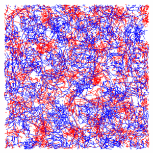
Figure 6: The paths traced out by elliptic and hyperbolic points in a chaotic flow. Can their trajectories be described mathematically?
Gollub and Ouellette's results are an interesting marriage of experiment and sophisticated mathematical ideas, and they are a promising first step in a very interesting direction: describing a vastly complex physical scenario by a comparatively small number of geometric features. But there's much to do yet: "We haven't been able yet to express our results in a simple mathematical way. For example, over time our special points are wandering around in space making a complicated tangle of paths [see figure 6]. We would like to be able to express the dynamics of the fluids in terms of equations that describe these trajectories, at least statistically. This is a goal we have not achieved yet, and we don't even know if it's possible to do this."
The prospect of being able to replace the classical Navier-Stokes equations of fluid motion by a set of simpler equations describing the behaviour of geometric features will excite many fluid dynamicists. So is Ouellette and Gollub's discovery something of a revolution? Gollub restricts himself to calling it a "worthwhile path for future study. We usually are very poor at predicting the significance of scientific or mathematical advances. I have no idea whether our work will prove to be important. And that's not a motivation for doing this kind of work. We do it because it is interesting and there is something of physical beauty in the shapes and forms we are studying and in the connection between physical phenomena and mathematics. Whether it turns out to be useful is something we can hope for, but not expect."
About this article

Marianne Freiberger, Co-Editor of Plus, interviewed Jerry Gollub at the Centre for Mathematical Sciences in Cambridge in January 2009. Jerry Gollub is Professor of Natural Sciences (Physics) at Haverford College, and Leverhulme Visiting Professor at the University of Cambridge.
Nicholas Ouellette was Research Associate in Physics at Haverford College before assuming his present position as Assistant Professor of Mechanical Engineering at Yale University.