The Arctic ice cap is in trouble. Due to global warming, summer sea ice cover has been disappearing at approximately 70,000 km² per year, an area the size of Scotland. Measurements from submarines indicate that the ice has grown thinner by at least 40% over the last two decades. Predictions of if and when the permanent ice will disappear from the Arctic vary widely, but few models give it longer than 100 years and many predict that a total melt-down of the Arctic will occur within our lifetimes.

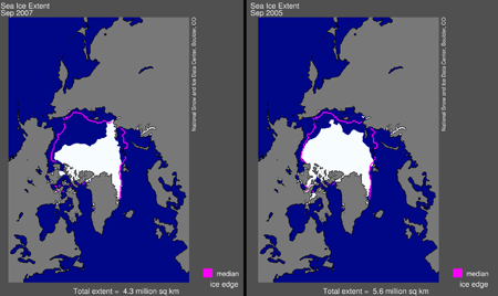
This image compares the average sea ice extent for September 2007 to that of September 2005. The magenta line indicates the long-term median from 1979 to 2000. This image is from the NSIDC Sea Ice Index.

This is not just troubling news for the North Pole. "There is a lot of feedback between Arctic sea ice and climate systems in general," says Peter Wadhams, Head of the Polar Ocean Physics Group at the University of Cambridge. "As the ice area decreases you're replacing an area of white, which reflects about 90% of the solar radiation, by open water, which reflects less than 10%. As the sea ice retreats you're absorbing a lot more radiation and this increases the rate of warming at high latitudes." This effect can raise the global average rate of warming by 20%.

And there are more knock-on effects. The marine eco-system will change dramatically with many species, from the Polar bear to tiniest bacteria and zoo plankton, facing extinction. Melting areas of permafrost will release trapped greenhouse gases like methane — this effect has already been observed in the Pacific Ocean and on the Siberian continental shelves — driving on global warming. As surface temperatures increase, more ice will melt and sea levels rise.

Sea ice also helps drive the Gulf Stream, the ocean current responsible for the mild climate in North-Western Europe. As the ice forms in areas of the central Greenland Sea, it rejects salt, creating a layer of high-density water. This water then sinks and the resulting convection gives rise to a global ocean current system known as the Great Ocean Conveyor Belt. If the ice fails to form, the Gulf Stream could slow down. "Some of the implications of an ice free Arctic haven't even been dreamed up yet," says Wadhams, "The modelling of the impacts is still in quite a primitive state."

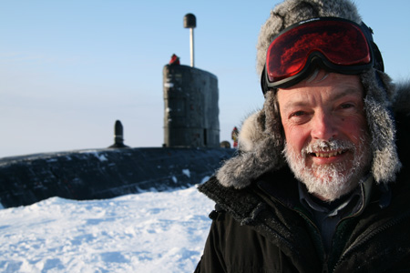
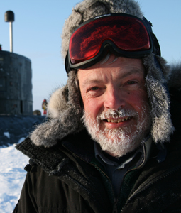
Peter Wadhams and one of the submarines that takes him below the ice.

If the recent warming in global temperatures is human-made — as scientists now accept — it's ironic to note that an ice free Arctic will provide new opportunity for human intervention. In the summer the Arctic will become accessible to oil exploration and fishing, and act as a shipping short-cut between Europe and Japan. Geo-political conflict may well be on the cards.

To prepare for the effects of climate change, not to mention to try and halt or even reverse them, we need to know for how long the Arctic ice cap will be around, and we need to know it fast. Mathematical modelling of sea ice behaviour can provide this much-needed glimpse into the future. And although comprehensive ice-ocean-climate models are complex beasts indeed, some relatively simple maths can give us a glimpse of the kind of challenges that scientists face.

How does ice grow?

Sea ice is subject to a huge range of influences: air and water temperature, ocean currents and wind, to name but a few. But let's leave reality aside for the moment and ask some very simple questions. How would a layer of ice behave if temperature was the only factor to consider? How fast would it grow and is there a limit to the thickness it can reach?

Figure 1: A simple model of ice growth.

To build a simple model, imagine a round slab of ice of uniform thickness and surface area of, say, 1m² floating on a column of water. Above the ice we have a column of air. We'll assume that the air has a constant temperature below the freezing point of sea water. The temperature of the water below the ice is of course above the freezing point. Now the warmer sea water will transfer energy through the ice into the air above in the form of heat, measured in joules. Letting $Q$ stand for heat and $t$ for time, Fourier's law of heat conduction tells us that the rate of heat transfer is given by the differential equation \\ \\ $ \;\;\;\; dQ/dt = \frac{k (T_w - T_a)}{h},\;\;\;\;\;\;\;\; (1) $\\ \\ where $k$ is the thermal conductivity of the ice, $h$ is the thickness of the ice, and $T_w$ and $T_a$ are the temperatures at the ice/water interface and the ice/air interface respectively. We'll assume that the latter two values remain constant as time passes.

As the sea water below the ice loses heat, some of it — a layer on the water surface — will freeze. There is a simple linear relationship between heat loss $Q$ and the mass $m$ of the layer: $$Q = Lm,$$ where $L$ is the latent heat of sea water, in other words the amount of heat loss required to freeze 1 kilogram of it.

Now the mass $m$ of a layer of water is equal to its density $D$ times its volume $V$. Density varies with temperature, but we will assume that in a thin layer close to the ice/water interface temperature is constant (around freezing point). Since a cross section of our water column has surface area 1, we have that $Q$ is equal to $L$ times $D$ times the height of the layer.

Thus, as the water loses $Q$ joules in heat through the ice layer, the ice thickness $h$ grows by an amount $Q/LD$, giving $$dh/dQ = 1/LD.$$ Combining this with equation (1) above, we get the differential equation $$dh/dt = \frac{k(T_w-T_a)}{LDh}.$$ A solution to this is the function $$h(t) = \sqrt{h_0^2 + \frac{2k(T_w-T_a)t}{LD}},$$ where $h_0$ is the initial thickness sof the ice layer. Don't worry about the various constants in this expression. The important bit of information is the fact that ice thickness grows with time $t$ like the square root of $t$.

Despite its simplicity, the model picks out some of the main features of ice growth. As the ice thickness $h$ increases, the rate of growth slows, reflecting the fact that cracks in the ice will try and "heal" themselves by growing faster than the surrounding thicker ice. An ice field of varying thickness will try to become level as thin ice grows more rapidly than thick ice. The first mathematical model for the growth of young ice, formulated in the 1890s by Josef Stefan, does in fact predict exactly this kind of ice growth.

Since Stefan's time, scientists have refined thermodynamic models to take account of more factors, including, for example, the effect of solar radiation. A standard model used by scientists today was developed by Maykut and Untersteiner in the 1970s. It predicts that if left alone for years, the ice approaches an equilibrium thickness of 2.88 metres, around which it oscillates on a seasonal basis.

Ice on the move

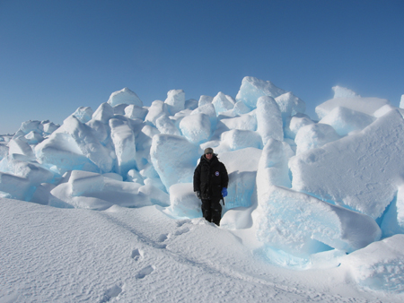
Ice fields often resemble rubble fields with randomly heaped blocks of ice.

So far we have completely ignored that sea ice is in constant motion. Winds tear at its surface and it is driven by ocean currents. The ice responds to these stresses with cracks and pressure ridges, which in turn change its response to wind and ocean.

It's a complicated business, but again a relatively simple model can get us quite far. To understand how ice motion depends on external forces, we turn to Newton's second law of motion, which states that the acceleration of an object is equal to the net force acting on it divided by the object's mass.

So let's take a piece of ice of area, say, 1m². The net force at work here comes from the various stresses acting on the ice, which clearly include air stress, due to wind, and water stress, due to currents. But another factor we can't ignore is the fact that all our measurements are made with respect to the Earth, which is itself in motion. This gives rise to what is called the Coriolis force (see the Plus article Galloping gyroscopes for an explanation). It's negligible on a human scale, but it plays an important role in sea ice motion, not least because its effect is strongest at the poles.

So we have $$Acceleration\; \times \;Mass = Air Stress \; + \; Water\; Stress \; + Coriolis \; Force, $$ which we write as $$\vec{a}m = \vec{\tau}_a + \vec{\tau}_w + \vec{\tau}_c. $$ Note that $\vec{a}$, $\vec{\tau}_a$, $\vec{\tau}_w$ and $\vec{\tau}_c$ are all vectors that encode the direction of the movement or force, as well as its magnitude.

Let's first turn to the stress exerted by the air. This is due to the air flowing around the ice floe dragging it along. In general the drag of a body in a flowing fluid is calculated using the equation $$\vec{\tau} = \rho C A |\vec{U}| \vec{U},$$ where $\rho$ is the density of the fluid, $A$ is the body's surface area, and $\vec{U}$ is the fluid's velocity. Again remember that $\vec{U}$ is a vector, and that $|\vec{U}|$ stands for the magnitude of a vector $\vec{U}$. The constant $C$ is called the drag coefficient of the body and it encodes the body's shape — a bulky body obviously reacts differently to the fluid flow than a flat and thin one. Note that the magnitude of the drag grows as a square of the speed of the airflow.

Figure 2: The wind drags the ice floe in the direction of U_a. As the ice moves in the direction of U_i, air resistance works in the opposite direction -U_i. Together we have the relative velocity U_a - U_i.

In our case the density becomes the density of air, $\rho_a$. Since ice fields often resemble rubble fields with randomly heaped blocks of ice, there's no easy formula for the drag coefficient $C_a$ of ice. Scientist usually assign it a value between 0.0014 and 0.0021, based on observations. We've assumed the surface area $A$ to be equal to 1.

Now if the ice floe itself is stationary, we get the equation $$\vec{\tau}_a = \rho_a C_a |\vec{U_a}| \vec{U}_a,$$ where $\vec{U}_a$ is the air velocity. However, we must take into account that the ice might itself be moving with a velocity $\vec{U}_i$, so rather than just $\vec{U}_a$ we'll use the relative velocity $\vec{U}_a - \vec{U}_i$: $$\vec{\tau}_a = \rho_a C_a |\vec{U}_a - \vec{U}_i| (\vec{U}_a - \vec{U}_i).

Water stress can be modelled in a similar way, this time with water density instead of air density, and with an underwater drag coefficient.

The Coriolis force $\vec{F}_c$ is given by $$\vec{F}_C = 2m \; \vec{\omega} \; \vec{U}_i sin \phi,$$ where $m$ is the mass of our piece of ice, $\vec{\omega}$ is the Earth's angular velocity, $\vec{U}_i$ is ice velocity and $\phi$ is latitude. The force's direction is 90 degrees to the right of $\vec{U}_i$ in the northern hemisphere and 90 degrees to the left of $\vec{U}_i$ in the southern hemisphere, a fact that has given rise to myths of water spiralling down plug holes in different directions on different ends of the planet.

What kind of motion does this model predict? Imagine that our floe of ice starts off perfectly still in the water until a sudden wind rises. Also assume, slightly unrealistically, that the water is not in motion, so that it only acts to slow down the piece once it is set in motion.

Figure 3: The air stress acting on the top of the floe is in the direction of the wind. The water drag is opposite to the direction in which the ice floe is moving. The Coriolis force is at right angles to the direction of movement (shown for the Northern hemisphere). The result is steady motion under a triangle of forces.

The force exerted by the wind will start moving the ice into the direction of $\vec{U}_a$. As soon as it has gathered sufficient speed, the Coriolis force will kick in, diverting its direction off to the right of the wind direction. The water drag will slow the floe, but as long as it is still accelerating, the Coriolis force will keep turning it. Eventually, as shown in the diagram, the direction of motion is far enough to the right of the wind for the Coriolis force, wind drag and water drag to balance in a perfect triangle of forces. The floe moves steadily at an angle of about 45 degrees to the right of the wind and at about 3\% of the wind speed.

This phenomenon was discovered by the famous polar explorer Fridtjof Nansen during the drift of his ship Fram across the Arctic in 1893-1896, and has become known as the Nansen rule.

Real ice bergs and floes have also been seen behaving like this. But still, reality is more complicated. We haven't taken into account that the water itself will move when a wind rises. Ice floes don't usually float about on their own, and the bumping and grinding in pack ice, for example, cause internal stresses that may well cause floes to break up. To model this you need a coherent theory of ice as a material. And to get a comprehensive ice-ocean model, you need to couple ice dynamics with thermodynamics.

More sophisticated models do exist however, and it is these that are fed into global climate models to predict the future of the whole planet.

The stats

There's another important component to ice-ocean modelling: statistics. Any mathematical model is built on observations and its predictions must be compared to real-life data. Many of the quantities that feed into the models, for example the drag coefficients, need to be estimated from observations. But collecting the necessary data is no easy task and requires statistical analysis.

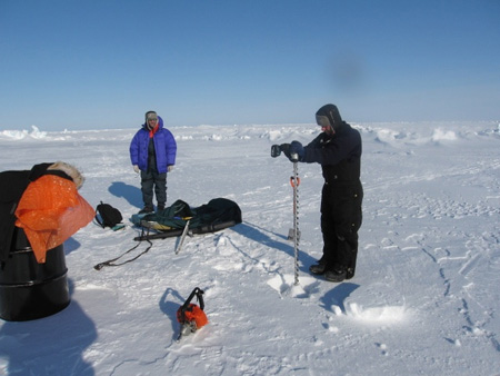
Hands-on work: Wadhams's team drilling a hole in the ice.

Satellites give scientists a good idea of what the surface of the ice looks like, but to get a picture of its underside — and its thickness — you need to get under the ice. Submarines with upward-looking sonar give valuable data, but only along the lines they follow. They only give a picture of a two-dimensional vertical slice of the ice. "It's a sampling problem," says Wadhams, "What we get from submarines is still not a perfect representation of the real distributions of ice thickness and features such as pressure ridges and open leads. When we're looking for trends in the data, we have an enormously difficult job assessing the statistical significance of our measurements and how representative they are of the ocean as a whole."

Wadhams and his team have indeed found that some features of the ice appear to follow regular laws. They found, for example, that the proportion of ice of thickness $h$ decays exponentially with $h$. "We don't know why," he admits, but spotting patterns like that can give vital clues about the processes — including wind, air and thermodynamics — that turn the ice into what it is. Let it be noted, at this point, that there is no doubt about the recent thinning of the ice: it is statistically significant and can't be put down to purely accidental factors.

A newly-developed multi-beam sonar and improved satellites will give more and better data in the near future, but to get a truly detailed data set, there's nothing but to go and see for yourself. In February 2009 a team of explorers will set out on foot on a 2000km journey from Point Barrow in Alaska to the North Pole (see Plus article The Arctic ice cap — how long has it got?). With them will be a surface-penetrating impulse radar that will measure ice thickness every 20cm along the journey. At the end of the journey, probably in June 2009, scientists from the Polar Ocean Physics Group in Cambridge, and from other institutions, will descend on the ten million or so readings to get the clearest picture of ice thickness to date.

Wadhams and his team regularly visit the Arctic and venture under the ice in submarines, as well as working from camps on the ice surface. Their next expedition is in May 2008, using an AUV (autonomous underwater vehicle), a kind of unmanned computer-controlled mini-submarine. It's not what you'd expect from Cambridge professors, but in these times there isn't the luxury to separate theory from practice. Arctic mathematicians may be a rare breed, but they're certainly not faced with extinction.

About this article

Peter Wadhams is Professor of Ocean Physics and Head of the Polar Ocean Physics Group based in the Department for Applied Mathematics and Theoretical Physics at the University of Cambridge. He is also a former Director of the Scott Polar Research Institute, also at Cambridge.

You can find out more about sea ice in Peter Wadhams's text book Ice in the ocean.