The Plus sports page: The curse of the duck

Eye on the ball
Cricket fans love their stats. Even the most casual follower can rattle off the batting averages of their favourite players or tell you how many wickets such-and-such a bowler took in the last test. The most passionate followers can recite each scorecard from this year's Wisden.
The recent news of the great Indian batsman Sachin Tendulkar surpassing West Indian Brian Lara's record number of test runs has given maths-loving cricket geeks another opportunity to pull out their calculators and Excel spreadsheets. I'm openly one of these nuts and did just that.
At the time of writing, Tendulkar had scored 12,027 runs across 247 innings, to overtake Lara's 11,953 from 232 innings. After a little investigation, I found that despite his outstanding average of over 54 runs per innings, Tendulkar's most common score in test cricket is ... zero!
This was quite a shock — the most prolific run-scorer in test cricket has been out for nought (a duck in cricket parlance) 14 times, well ahead of his second most common score — which incidentally is the next lowest you can get: one!

Donald Bradman was well known for his high backlift and lengthy forward stride.
This is completely counter-intuitive, so I took this investigation further. Australian cricketer Sir Donald Bradman is universally regarded as the best batsman ever to have played the game. His average, an astounding 99.94, is so far above every other batsman in the history of the game that he is often acclaimed as not only the best cricketer ever, but the best player ever of any sport. His average is so iconic in Australia that the postcode of the ABC (the Australian version of the BBC) is 9994 in every capital city. If it wasn't for the fact that much more test cricket is played nowadays than in the early 1900s, and for World War II interrupting his career for six years, Bradman would have scored many more than the 6996 runs he did score.
So, guess what Bradman's most common score was?
That's right, zero!
Indeed, looking at every innings by the most prolific batsmen in test history from Tendulkar at number 1 to Bradman at number 34, the most common score is zero — and by quite a long way too. The following figures show the distribution of scores from these top batsmen — on the horizontal axis you see the number of runs and the vertical axis measures the frequency of dismissals at a particular number of runs. The first chart shows every score between 0 and 100, and the second uses five-run wide bins to show scores up to 250. The data only include scores where the batsman was dismissed and so does not include not-out scores.

Scores plotted against dismissal frequency.

Scores in bins of five plotted against dismissal frequency.
Model cricket
A closer look at these distributions shows that they very closely fit what is known as an exponential distribution. An exponential distribution has the form $$y=\lambda e^{-\lambda x}.$$ In this case $y$ is the probability of being dismissed at score $x$ with $\lambda$ being a constant. A common trick when looking at distributions involving exponentials is to take logarithms of both sides to get $$ln(y) = ln(\lambda) - \lambda x.$$ The graph of this function, plotting $ln(y)$ against $x$, is now a straight line with slope $-\lambda$. If the statistical data fits the exponential distribution, then the plot of the logarithm of the frequency of dismissals against the score at which dismissal happened should look roughly like a straight line.

A straight line fitted to the data. The blue dots represent observed data and the black line represents the model.

A straight line fitted to the data from the second chart above. The blue dots represent observed data and the black line represents the model.
There is a very strong straight line fit in both charts. Using a standard technique called least-squares regression, we can find the straight line that best fits the data.We can determine $\lambda$ from the coefficient of $x$ in the equation of this line, and in our case this gives $\lambda$ equal to 0.023.
The mean of an exponential distribution, a sort of average, is $ 1/ \lambda$. In our case this gives a mean of around 43 - the same as we observe in the raw data. One can make the interesting observation that there is no such thing as the "nervous nineties": players do not "choke" and get out in the 90s, nervous before scoring a glorious test century, any more than they get out at any other score. Indeed, you could argue the opposite given the probability troughs at 94, 98 and in the 190s. You can also see that the probability of being dismissed for a duck is higher than you might expect for an exponential distribution.
So what?
Now, so far you might be thinking that all of this is only of passing statistical interest. So what if cricket scores follow an exponential distribution? Well, I'm glad you asked!
Let's turn for a second to a different distribution, the geometric distribution. You will be familiar with this distribution from a simple 50/50 coin toss. The geometric distribution describes the number of coin tosses you need before a head (or tail) first turns up. The probability of your first head turning up on your $kth$ toss is described as $$Prob(first\;\; head \;\; on \;\; kth \;\;toss) = (1-p)^{k-1}p,$$ where $p$ is the probability of a head turning up on each toss, that is, 0.5. The distribution is memory-less, which is one of its key descriptors. No matter what has gone before, even if you have fluked 100 tails in a row, the probability of a head turning up on the 101st throw is still $p$. The geometric distribution only works for integer values of $k$, that is, you can only throw a coin 2, 3, 100 etc times and not 2.5 times. The exponential distribution is the continuous equivalent of this distribution, extending it to work for all numbers, not just integers. Given that cricket batting scores seem to fit a exponential distribution, this means that we can picture cricket batting scores on a geometric distribution with the probability of you being dismissed at score $k$ as $$Prob(dismissed\;\;at\;\;score\;\;k) = (1-p)^kp.$$
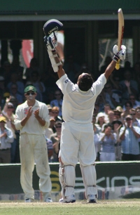
Sachin Tendulkar against Australia in the 2nd test at the SCG in 2008. Image by Privatemusings.
Can you spot the profound result here? Remembering that the geometric distribution is memory-less, you can interpret this as saying that no matter what score you are currently on, you have the same chance $p$ of getting out on that score as you do on any other score! Like a coin toss, the probability of you being dismissed on each score does not depend on what has gone before. A model which assumes that there is no memory is known as a constant hazard model. This seems to go against every cricketing manual I have ever read. Accepted cricketing wisdom says that a batsman is more dangerous when (s)he "has the eye in" and has scored 10 or 20 runs. Our result seems to suggest that, apart from when a batsman is on 0, you have just as much chance of dismissing him or her on the current score as on any other score. The next question to ask is, what is the probability of dismissing a batsman on the current score (that is, what is $p$ in the above equation)? The mean of a geometric distribution is $$mean = \frac{1-p}{p}.$$ Knowing that the mean of the exponential distribution is $1/\lambda$, and transferring this to the geometric distribution, we get $$p = \frac{\lambda}{\lambda + 1}.$$ For $\lambda = 0.023$ this gives $p = 0.022$. Therefore, if you were to turn the television on now and find the cricket coverage, the chance that the batsman you are watching gets out on the current score is 2.2\%.
Scores near zero
The biggest deviation from the geometric distribution is for scores near zero. According to our data, the chance of being dismissed for a duck is 6.9% — around 3 times more than expected for a geometric (or exponential) distribution. But by the time the batsman has scored two or three runs, the geometric distribution starts to fit well. There is a small peak at four runs, perhaps because you can relatively easily get to four before you become comfortable — it only takes one streaky shot to the boundary. Whilst you can get to three with one shot, you are more likely to have played a few shots and so may be comparatively more "set".

The data and the geometric distribution. The blue dots represent observed data and the black line represents the model.
An analysis of scores near zero has been completed by Brendon J. Brewer from the University of New South Wales in Getting your eye in: A Bayesian analysis of early dismissals in cricket. Brewer indeed found that batsmen are more vulnerable at the beginning of their innings.
By assuming a constant hazard model, Brewer determined the effective average of a batsman before they have scored — that is, assuming a constant hazard model with probability $p$ of dismissal equal to that of their chance of being dismissed for a duck, Brewer determined the mean of this new distribution.
In our data from the best batsmen of all time, dismissal for a duck occurred with a 6.9\% chance. The mean of a geometric distribution built around this probability is $$\frac{1-0.069}{0.069} = 13.5.$$ This means that even though our batsmen have a mean of about 43, before they've scored they bat like cricketers with a mean of 13.5. Even the best batsmen bat like tail-enders before they get off the mark!
Conclusions
What should we take away from this analysis?

Beware of the duck.
The conclusion seems to be that there is a very small window in the beginning of a batsman's innings in which there is a greater chance of dismissal than there ordinarily is. This makes sense — batsmen take some time to acclimatise to the game conditions. But this is a small window — once the batsman has scored about three runs, you have the same chance of dismissal whatever the current score. Interestingly, tiredness does not seem to play a part — the exponential distribution holds well out to 250 runs (quite a few hours of batting).
It should be remembered that this analysis was completed on the top 34 run scorers of all time (5953 innings) and so represents the best ever batsmen. Lesser batsmen are likely to get low scores, so perhaps this window is slightly wider for them. But if we turn to the greatest of the great, Bradman, the window is essentially one run. His effective average before he had scored was a very mediocre nine runs. After he had scored two runs, this effective average had risen to 69. You had to get Bradman out very early!
More information
- The data was retrieved from cricinfo during the second test between Australia and India on the 19th of October 2008;
- Not-out scores were removed from the analysis;
- The exponential distribution does break down a little for scores above 250 as there simply isn't enough data;
- Yes, Marc has scored a duck in his cricket career.
Further reading
- Read Brendon J. Brewer's paper Getting your eye in: A Bayesian analysis of early dismissals in cricket;
- Find out more on the maths/cricket blog Pappus' plane — cricket stats.
Previously on the Plus sports page
Marc West is a freelance science writer and former Assistant Editor of Plus who currently works in operations analysis in Sydney.
As a wannabe Australian cricket player, the stars aligned when Marc somehow scored 114 against Mount Colah in a Sydney shires cricket game. He loves to write about science and sport and has been published in a variety of magazines and newspapers. You can read more of his writing on his personal blog.