Supersonic Bloodhound
Back to the Constructing our lives package
The land speed record
The first vehicles that today we might describe as cars were steam powered and used primarily for transporting large heavy loads back in the 18th century. Ever since, engineers have been pushing boundaries to try and get them to go faster. The first official land speed record was set in 1898 by a French chap called Gaston Chasseloup-Lausat. He reached the mind-boggling speed of...
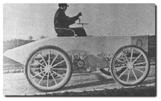
The first ever land speed record was set by Gaston Chasseloup-Lausat.
...39mph!
We've come a long way over the last century; steam driven vehicles have been replaced by electric vehicles, electric vehicles have been replaced by piston engine vehicles, and now jet and rocket powered vehicles are the dominant force in the world of super-speedy cars. Over the last few decades, there has been a ding dong battle for the record between the Brits and the Americans, but Britain has now held the record for over 25 years. Britain currently holds the only supersonic land speed record with Thrust SSC driven by Andy Green, 763mph! (You can read an interview with Green in this issue of Plus.)
And now we want to push things even further. The Bloodhound project, spearheaded by ex-land speed record holder Richard Noble, aims to take a car up to the dizzy heights of 1,000mph, about 1.3 times the speed of sound! At these speeds the forces generated by the aerodynamics are huge. In parts, the car surface will experience pressures up to 12 tons per square metre. That's like having a large elephant come and sit on your chest! So, before we build the car we have to use computational fluid dynamics to try and predict how it will behave. "But what on earth is computational fluid dynamics?" I hear you ask! Don't worry, we will come on to that.
Computational fluid dynamics
Mathematicians have been forming and solving equations for centuries. In fact, we have evidence that human beings have been solving equations as far back as 2000 BC, when the Babylonians were the dominant world superpower. We have come a long way, over the centuries, in our abilities to solve equations. And that is a good thing, because more often than not it is a brand of equations called differential equations that are at the heart of descriptions of natural processes, including the spread of diseases, the weather, climate change, or lightning strikes. Differential equations involve the rate of change of variables or derivatives. They are the most common equation type that describe nature but, unfortunately, they are not the most straightforward to solve.
Newton was developing techniques for solving these tricky equations in the eighteenth century, but the full power of the techniques he developed could not be exploited until the advent of the computer in the last century. Now, with the most powerful computers in the world, we can solve some of the trickiest equations in the world, including the equations that describe airflow, known as the Navier-Stokes equations. You can see (below) that when they are written out in full they are a bit of nightmare to say the least! It's simply not going to be possible to get out a pen and paper and sit down and solve them analytically. We're going to need some help, and that's where we turn to a supercomputer. (You can read more about the Navier-Stokes equations in the Plus articles listed below.)
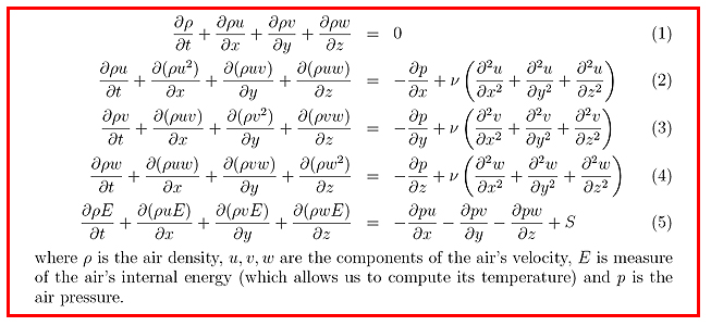
The Navier-Stokes equations.
But where do these equations come from? Actually, their origins are quite straightforward. The first equation originates with the principle of conservation of mass, which says that mass can neither be created nor destroyed. The second, third and fourth equations come from the principle of conservation of momentum in the three spatial directions x, y and z, and hence they look very similar. The principle states that the rate of change of momentum of a system must be equal to the applied force. The final equation stems from the principle of conservation of energy, which says that energy can be neither created nor destroyed, only converted from one form into another.
So where do you start when trying to solve a set of equations like this? Like all complex problems, we have to break it down into smaller, more manageable chunks. And the method employed is known as the finite element method. In essence, we divide the space surrounding the car into a massive assortment of very small elements (100,000 million of them!). We call this a mesh. Then we tackle the problem element by element, each element making a simplified approximation to the solution across it, and with each element in constant discussions with its neighbours, until we have the complete solution. From this solution we get the air density, air velocity, air temperature and air pressure at all points surrounding the car.
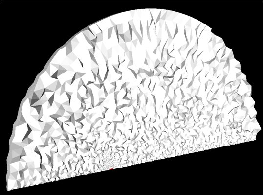
A mesh for solving the Navier-Stokes equations.
Once we know how the pressure over the vehicle varies as it accelerates up to its top speed, we can use integration to sum up the effects of this pressure over the vehicle and work out the total forces. The procedure is very similar to the trapezium rule, which estimates the area under a curve by approximating it by trapezia, and then summing their areas.
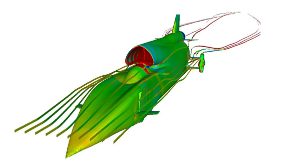
Pressure contours and streamlines over Bloodhound SSC.
Using computational fluid dynamics, we are answering questions such as "How much drag will the car experience?", and "Will it stay on the ground at all speeds?". These are the questions that have driven the design process of the car and ultimately given the car its external shape.
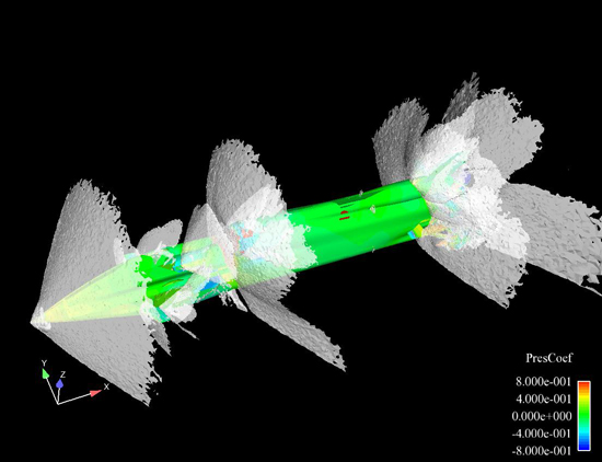
Bloodhound SSC at Mach 1.3, coloured by pressure coefficient showing the position of shock waves.
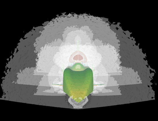
Another view of Bloodhound SSC at Mach 1.3, coloured by pressure coefficient showing the position of shock waves.
The design of Bloodhound SSC
By combining the predicted aerodynamic forces with the anticipated weight of the vehicle and the predicted thrust from Bloodhound's jet and rocket propulsion system, we are able to predict exactly how the car will behave. And the results are quite spectacular. It will cover 10 miles in approximately 90 seconds, reaching a peak acceleration of +2.5g, increasing in speed by 60mph every second, and peak deceleration of -3.0g. At its top speed it will cover a mile in 3.5 seconds!
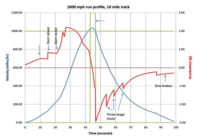
A 1000mph record run profile indicating velocity and acceleration against time.
None of this would be possible without the use of mathematics. As things stand, the maths tells us that 1,000mph is possible...
But whether or not we, the Bloodhound team, can convert theory into practice is a question that will only be answered after a fascinating adventure. So watch this space!
You can find out more about the Navier-Stokes equations in the Plus articles How maths can make you rich and famous, Understanding turbulence, Universal pictures, and Births and deaths in fluid chaos.
About the author
Dr Ben Evans studied Aerospace and Aerothermal Engineering at Jesus College, Cambridge graduating in 2004. After graduating, he immediately began a PhD in Computational Fluid Dynamics at Swansea University which was completed in October 2008. In his PhD research he focussed on computational solutions to problems in the field of molecular gas dynamics.
Dr Evans began working as a research assistant under the supervision of Professor Oubay Hassan in the summer of 2007. His post-doctoral research was on the development of unstructured mesh techniques for high speed flows with particular application to the Bloodhound supersonic car.
Comments
David Harold Chester
I have been trying to impress the Bloodhound team with the importance of investigation of the instability of rotating wheels on a surface, otherwise known as shimmy or wheel flutter. As an aerodynamicst you might be able to introduce them to this subject as a wheel flutter situation, due to the supersonic air-speeds and forces around the wheels (as well as the mass and stiffness contributions to the dynamics of this motion). I see this problem as needing a solution before high-speeds are reached, so that the potential risks are minimized and the shimmy boundaries properly defined.
Karan Aggarwala-PhD
Computational math of turbulence to create models for high-speed cars and for aviation gains elegance of graphical representation if we divide the quadrant into 63 wedges and the half circle into 126 narrow triangles.