Measuring catastrophic risk
The notion of uncertainty
In the early 19th century, the French mathematician Pierre-Simon de Laplace wrote of a concept he had been thinking about for some time. The concept became known as Laplace's demon and was a thought experiment which sought to clearly explain the existence of uncertainty. It is described in his Essai Philosophique sur les Probabilités (1814) as:
"An intellect which… knew all the forces that animate Nature and the mutual positions of the beings that comprise it, if this intellect were vast enough to submit its data to analysis, could condense into a single formula the movement of the greatest bodies of the universe and that of the lightest atom: for such an intellect nothing could be uncertain; and the future just like the past would be present before its eyes".
This is quite a powerful idea. If there existed a being (or a model in our case), with infinite knowledge and processing capability, we could perfectly predict the future. In other words, there would be no uncertainty. This experiment illustrates quite clearly why all models must encompass some form of uncertainty, since we do not have infinite levels of knowledge and processing power. Catastrophe models, also known as cat models in the insurance industry, are no different (for a description of catastrophe models, see my Plus article Modelling catastrophes). The purpose of catastrophe modelling is to anticipate the likelihood and severity of catastrophes so that companies and governments can appropriately prepare for their financial impact. There is a lot of uncertainty involved here: not only do we not know exactly when a catastrophe might occur, we also don't know how much damage it will inflict. As figure 1 below shows, the amount of damage caused by a hurricane to buildings of a similar type can be quite varied, even when they are subjected to the same wind speed (the damage ratio in the below graph represents the proportion of a building that is damaged).

Figure 1: Graph showing variation in damage from a hurricane (main) and an illustrative picture of two identical adjacent buildings which can experience different levels of damage (inset) at the same windspeed.
Uncertainties in models
The uncertainty arising from natural processes can be grouped broadly into two types: aleatory and epistemic uncertainty. The word aleatory is derived from alea, Latin for a game of dice, and this type of uncertainty represents the intrinsic variability of a process. Epistemic uncertainty, whose name is derived from the Greek word epistemikos, meaning knowledge, stems from a lack of understanding of the true behaviour of a process. In catastrophe models, uncertainty can arise in a variety of ways; from uncertainty in the time of occurrence of earthquakes on a fault (aleatory) to uncertainties surrounding the behaviour of sea surface temperatures in the near future and their impact on landfalling hurricane risk (epistemic). Cat models attempt to quantify these uncertainties in two main ways: by simulating a catalogue of events, for example a catalogue of tropical cyclones, and by measuring the uncertainty surrounding the amount of damage caused by each simulated event. We'll have a more detailed look at both of these below.
Risk Metrics
Catastrophe models can help companies protect themselves against insolvency by providing information on the likely yearly loss and extreme catastrophic losses. Figure 2 below shows the probabilities of varying amounts of loss/profit, with and without financial protection, such as insurance. We see that protection reduces profit/loss volatility (represented by the narrower shape of the blue curve ) and also protects against large losses (as can be seen by the negligible probability of a large loss for the blue curve). The price for this protection is that the possibility of larger levels of profit is sacrificed.

Figure 2: Expected net earnings, with and without financial protection.
The stock market crash of 1987 led to an increased focus on ways of measuring risk, or risk metrics. One reasonable question to ask is: "given an amount $L$ of loss, say 1 million dollars, what is the probability that a company will incur that loss of $L$, or larger, over the coming year?" However, it also makes sense to ask the question the other way around: "given a chosen probability, say 0.004 or 0.4\%, what is the value of loss $L$ such that the probability of incurring a loss of $L$ or larger is equal to the chosen value of 0.004?" This value of $L$ is called the Value at Risk (or VaR) — in our example it's the 0.4\% VaR. The VaR is a measure of the risk posed by extreme events: the probability of the yearly loss occurring is small, only 0.4\%, but the VaR gives you an idea of how dramatic its impact will be if it does indeed occur.
Incidentally, in the same year as the crash, the field of catastrophe modelling was created — see the article In nature's casino by Michael Lewis in the New York Times. The metric of choice that emerged for monitoring risk in cat modelling was Value at Risk, although the name used was probable maximum loss (PML), and means the loss at a specified exceedance probability.But how can we determine such metrics, given that we don't know if and when a dramatic event is going to strike? The answer comes from stochastic models of natural processes. These mathematical models capture the physics of a natural phenomenon, as well as the uncertainties involved. Using such models, it is possible to simulate a large catalogue of events, for example 10,000 scenario years of tropical cyclone experience. Each of the 10,000 years should be thought of as 10,000 potential realisations of what could happen in the year 2010 for example, and not simulations until the year 12010.
For each simulated year, you can then work out the damage the event would have caused to, say, a set of buildings, and then rank the simulated years by their total loss. This information can then be displayed in the form of an exceedance probability curve, shown in figure 3, which is a plot of the VaR against the corresponding probability for a notional set of risks.
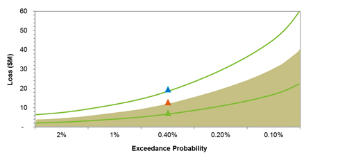
Figure 3: Graph showing the exceedance probability curve for a notional set of risks, together with the associated 5th and 95th percentiles (see below for an explanation).
As an example, the 40th largest loss, call it $L$, in a 10,000-year catalogue will be the loss at an 0.4\% exceedance probability: this is because a loss of $L$ or larger occurs in 40 out of 10,000 simulated years and 40/10000=0.004, which equates to 0.4\%. The inverse of the exceedance probability percentage gives the return period, that is, it tells you how often an event is expected to occur: for a 0.4\% percentage probability, the return period is 1/0.4=250, so the event is expected to occur once in 250 years.
There is, however, another level of uncertainty that needs to be captured: even if we do know the chance of an extreme event (like a hurricane) occurring, we cannot be sure exactly how much monetary loss the event would cause (since houses react to hurricanes differently). However, past experience with extreme events (eg using losses incurred by actual events) makes it possible to come up with a probability distribution telling you the chance that the financial damage caused by a given event takes on specific values. This information can be included in the exceedance probability curve. For example, figure 3 tells us that there is a 0.4% chance that the mean total loss in one year would be $11m or greater. However, the figure also gives the 5th and 95th percentiles, $7m and $19m for a probability of 0.4%, which are represented by the two green curves. These give the lower and upper bounds of a 90% confidence interval: although the loss may not be exactly $11m, we can be 90% confident, given the assumptions of our model, that it will lie between $7m and $19m.

Hurricane Isabel (2003) as seen from the International Space Station. Image courtesy NASA.
The exceedance probability curve helps to inform opinions on the management of risk: using robust risk metrics, together with their correct interpretation, is fundamental to making good business decisions.
Nevertheless, just looking at a single metric is not advisable. Taking on new business may largely change the behaviour of low frequency risk on the existing portfolio and also add new risks if it involves locations where extreme events are more likely to occur. New business can be the selling of a contract obliging the insurer to pay all US wind damage incurred by any branches of a particular company in exchange for a premium. Existing business is the combination of all risks whose losses the insurer has currently agreed to cover. One metric that is used to monitor low frequency risk, also known as tail risk, is Tail Value at Risk or TVaR. The TVaR represents the average of all the losses that are greater than the loss at a specified exceedance probability. For example, for a 10,000-year catalogue and an exceedance probability of 0.01, the TVaR is the average of the top 100 annual losses as simulated by the model. (In finance the TVaR is also known as expected shortfall.)
(Mis)interpretation of risk metrics
The old adage "Don't put all your eggs in one basket" applies here, since risks should be spread widely to prevent any single occurrence from having a dire effect on a company's profitability and solvency. Hence, when checking the impact of new business on the existing portfolio of an insurance company, the change in the loss at a specified exceedance probability is an important metric (this is known as the marginal impact of the new business on the current portfolio). That is, at the same exceedance probability $p$, the VaR $L_{p}(E+N)$ is calculated for the existing business $E$ and new business $N$ combined. This is a quick check to see whether a set of new risks helps diversify the current portfolio or adds more risk than there currently is appetite for.
The risk associated to two portfolios combined clearly can't exceed the risks of the two separate portfolios added together, and any decent risk metric should reflect this. In technical terms, any risk metric $R$ should be sub-additive: $$R(E+N) \leq R(E) + R(N),$$ where $E$ and $N$ stand for existing and new business respectively.
This seems like an obvious requirement, but it turns out that metrics based on exceedance probability alone, like the VaR, do not not always satisfy it. The TVaR, however, emerges as one metric which obeys the sub-additivity rule.
What is more, TVaR information, as opposed to information that only uses the loss at a given exceedance probability, can give further insight into the potential loss from a set of risks. This is illustrated in figure 4 below, which shows risk profiles for a single location for both earthquake (EQ) and tropical cyclone (TC) perils. The left panel shows the loss plotted against return period and the right panel shows TVaR plotted against return period. Recalling that the return period is the reciprocal of exceedance probability, we note two things: firstly, for this location, years with loss causing earthquakes are less frequent than years with losses from tropical cyclones. We can see this as losses only appear at return periods greater than 1000 and thus for the 10,000 year catalogue there are less than 10 loss causing years. Secondly, when earthquakes do occur the loss potential is more significant than for tropical cyclones. At the 3,000 year return period (or 0.033% exceedance probability) we might conclude that the risk of both perils is the same, however this is patently mistaken when we look at the TVaR metric (right panel). Consequently, TVaR can be thought of as a more robust metric to the quantification of tail risk.

Figure 4: Comparison of different risk profiles for a single location between earthquake and hurricane perils.
Conclusion
Uncertainty is ubiquitous. We see it every day in weather reports, traffic forecasts, book-keeping odds, and even in the forecast of where a hurricane will make landfall hours in advance. The strength of catastrophe models lies in their ability to show holistically the uncertainties present in the modelling of extreme events, and their loss potential. Following from this, risk management needs to be undertaken based on the understanding of the strengths and limitations of the associated risk metrics; this will aid in more accurate risk management practices.
You can read another article on catastrophe models on the Understanding Uncertainty website.
About the author

Shane Latchman works as a Client Services Associate for the catastrophe modelling company AIR Worldwide Limited. Shane received his BSc in Actuarial Science from City University and his Masters in Mathematics from the University of Cambridge, where he concentrated on probability and statistics. Shane is keenly involved in getting non-catastrophists interested in the catastrophe modelling industry and regularly gives talks and writes articles on the topic for both an industry and non-industry audience.
Comments
Anonymous
What do negative TVaR values signify?