Police and thieves

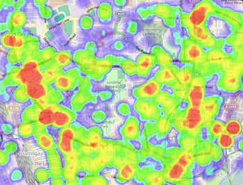
A map of crimes committed in an area of North London in 2012. The red regions are hotspots. Image from the UK Crime Heat Map.

When the mathematician Andrea Bertozzi started her new job at the University of California, Los Angeles, in 2003 she decided to use her skills to study a problem that has plagued LA for a long time: crime.

Crime is a problem in most cities, but as we all know, not all neighbourhoods are affected in the same way. There are crime hotspots you wouldn't want to enter alone on a dark night, or even during the day. It's clear that all sorts of factors contribute to turning an area into one of those: for example its socio-economic standing, or the density of the population. It would be useful to get a clearer understanding of the dynamics of hotspots. This is where maths can help. You can try to describe the processes involved using mathematical rules and equations — build a mathematical model — and see what this simplified version of reality tells you about what's going on.

Criminal games

One model Bertozzi and her colleagues have worked on starts with the basic components of any crime: the criminals and their targets. The team came up with a way of simulating burglary patterns, which you can think of as a computer game in which virtual criminals march through a grid of virtual houses. At every time step (say each day or each hour) each criminal finds itself at a particular house and decides whether to break in or not. If it does break in, then it disappears from the grid in the next time step, as burglars tend to make off with their loot straight away. If it doesn't, then it moves on to appear at an adjacent house in the next time step.

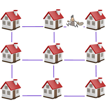
A grid representing an area of a city.

The decision of whether a burglar breaks into a given house is made by chance, but not necessarily a 50:50 chance. For each house there's a probability that a burglar will enter at a given point in time. That probability depends on an attractiveness value of the house at that particular time — and that value is chosen to reflect what you know about crime and criminals' behaviour in the area you are trying to understand.

The probability of burglary

The probability that a burglar located at house $H$ between times $t$ and $t+\delta t$ breaks into the house is

$p_ H(t) = 1-e^{-A_ h(t)\delta t}.$

This probability comes from what is known as a Poisson process, used to understand the occurrence of events over time.

We’ve already mentioned that factors like socio-economic situation, population density, or even the traffic volume of an area are linked to the amount of crime that happens there. To reflect that, each virtual house $H$ in the model comes with a number $A_ H$ which measures how likely it is to be burgled simply because of the areas it’s in. But crime statistics also show that criminals like to build on their success: if a house has just been burgled, then the chance that it, or its neighbours, will soon be burgled again goes up. Therefore, in our computer game, each house $H$ also comes with a number $B_ H(t)$ which reflects recent criminal activity: it increases if there’s just been a break-in at $H$ or one of its neighbours, but then gradually decreases as time $t$ goes on, until the next crime happens there. The overall attractiveness of house $H$ at time $t$ is

$A_ H(t) = A_ H + B_ H(t).$

The probability $p_ H(t)$ that a virtual burglar breaks into house $H$ at time $t$ depends on the attractiveness value: the greater $A_ H(t)$ the greater $p_ H(t)$ . (You can see the precise relationship in the box above).

Moving on

The probability that a burglar moves from house $H$ to adjacent house $G$ at time $t$ is

$q_{H \rightarrow G} = \frac{A_ G(t)}{S_ H(t)},$

where $S_ H(t)$ stands for the sum of the attractiveness values of all the houses adjacent to $H$ at time $t$ .

If the burglar doesn’t break in, then it needs to decide where to move on to. Again this decision is made by chance and governed by probabilities which compare the attractiveness value of one adjacent house to the attractiveness values of the other adjacent houses (the exact formula is in the box on the left).

The simulation now works like this. At each time step the burglary probability $p_ H(t)$ is calculated for each house $H,$ based on the attractiveness value $A_ H(t).$ Burglars then either break into the house they're at or move on, their actions governed by the appropriate probability. Then the attractiveness value for the next time step is calculated. To do this, you need a formula for the $B_ H(t)$ which reflects how recent criminal activity effects a given house. The formula is a little more complicated, but you can see it here. Also, at each site in the grid new burglars are generated at a rate $N,$ as otherwise all burglars would eventually disappear. Then the loop starts again for the next time step.

What do the simulations tell us?

The simulation depends on a number of parameters, such as the intrinsic attractiveness $A_ H$ of a house, the rate $N$ at which burglars are generated, another quantity that measures by how much the probability a housed gets burgled increases after a recent burglary, and so on. If you want to use the simulation to get an idea of crime in a particular area of a real city, you need to estimate those parameters by looking at the data you have available.

When Bertozzi and her colleagues ran the simulation for different sets of parameter values, they saw three distinct patterns emerge. In one of them the attractiveness of houses, and therefore the burglary pattern, is more or less the same across the whole area that's being simulated. In the second, crime hotspots emerge where the attractiveness value of houses is high compared to houses not in the hotspots. The hotspots remain for varying amounts of time; they can stay in one place but also move around. In the third, hotspots also emerge, but they stay put: the whole system becomes stable in the sense that not much changes over time.

But what can we learn from this mathematical model? Find out on the next page.

About this article

This article was inspired by Andrea Bertozzi's Rouse Ball Lecture, which took place in Cambridge in April 2015.

Marianne Freiberger is Editor of Plus.

Comments

How can I assess or calculate

How can I assess or calculate the AH number?

Plus.Maths.org