
Catching waves with the Laplacian
Brief summary
The Laplacian operator turns up all over maths. Here's a reasonably light-touch introduction and a look at why it forms part of the wave equation.
When you pluck a guitar string or bang a drum you hear a sound. That's because your action causes the string, or the membrane of the drum, to vibrate. The vibrations send packets of low and high pressure travelling through the air. It's when these sound waves hit your eardrum that you perceive the sound.
Describing this process mathematically takes a good understanding of physics and some calculus. In this article we will give a light-touch, and relatively intuitive, overview that combines both the physics and the maths, but hopefully without leaning too hard on your understanding of either. If you understand derivatives and have a bit of physical intuition you should be fine.
The Laplacian
Key to the mathematics of sound is something called the Laplacian operator, named after the mathematician Pierre-Simon Laplace. The Laplacian operator is often denoted by $\Delta$ or by $\nabla^2$. For simplicity, we will stick to $\Delta$. The operator takes mathematical functions of spatial variables as input and returns the sum of their (unmixed) second partial derivatives as output.
If you are looking at a function of one variable, $f(x)$, then the Laplacian operator simply returns the second derivative:
$$\Delta f = \frac{d^2f}{dx^2}.$$
If you're looking at function of two variables, $f(x,y)$, then
$$\Delta f = \frac{\partial^2 f}{dx^2} + \frac{\partial^2 f}{dy^2}.$$
Generally, for a function of $n$ variables, $f(x_1, x_2, …, x_n),$ we have
$$\Delta f = \frac{\partial^2 f}{d{x_1}^2} + \frac{\partial^2 f}{d{x_2}^2} + ... + \frac{\partial^2 f}{d{x_n}^2}.$$
What does the Laplacian tell us?
Let's stick to the example of a function of one variable, $f(x)$. To make things look a little neater we write $f'(x)$ for the first derivative and $f''(x)$ for the second derivative.
The first derivative $f'(x)$ gives the rate of change of the function at the point $x$. In other words, it gives us the slope at $x$. When the first derivative is equal to $0$ at $x$, then $x$ is a minimum, a maximum, or an inflection point.
The second derivative at $x$ measures the rate of change of the slope at $x.$ If it's not zero, then $x$ is a maximum or a minimum. In this case, the larger the absolute value of the second derivative at $x$ the more dramatic the change in slope and the more extreme the bend of the curve at $x.$
To see this, look at the examples $f(x)=x^2$ and $g(x)=2x^2$. The second derivatives evaluated at the point $0$ are
$$f''(0) = 2$$ and
$$g''(0) = 4.$$
And as you can see from the graphs, $g$ is a lot more curved at $0$ than $f$.
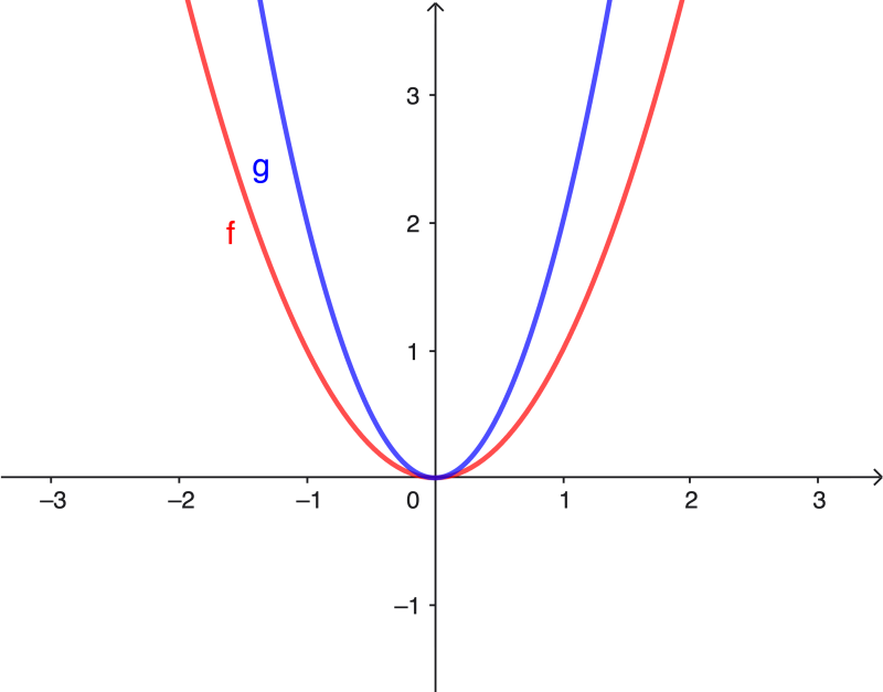
This suggests that the second derivative can be used to measure the curvature of the graph of $f$ at $x$, at least as long as the slope (the first derivative) at $x$ is zero or very small.
And this is indeed true. The geometric curvature $k$ of a curve given by a function $f(x)$ is defined as
$$k=\frac{|f''(x)|}{(1+(f'(x))^2)^{3/2}}.$$ When $f'(x)$ is near $0$ then $k$ is approximately $f''(x)$.
Another thing to note is that if the curvature at a particular point $x$ is high, then this also means that $f(x)$ differs quite a bit from the average value of $f$ at nearby points: that's because the curve bends sharply away from $f(x)$. This intuition can be made precise (there's quite a nice explanation in this video), so it turns out that the Laplacian can also be thought of as giving information about how much $f(x)$ deviates from the local average.
The intuition also works for a function of two variables whose graph is not a curve, but a surface. Such a surface can model the membrane of a drum, which vibrates when you bang it.
What's a wave?
Now let's go back to the vibrations in a plucked string. Let's think of the string when it's at rest as a horizontal line. We can think of the line as part of the $x$-axis of a 2D Cartesian coordinate system.
The movement of the string or drum can be described in terms of the displacement $u(x,t)$ which the string experiences at point $x$ and time $t$. This is best explained with an animation:
The first derivative $\frac{\partial u(x,t)}{\partial t}$ with respect to time tells us how fast the point on the string moves.
The second derivative $\frac{\partial^2u(x,t)}{\partial t^2}$ with respect to time tells us the acceleration of the point.
Newton's second law of motion has something to say about the acceleration an object experiences when acted on by a force: it is equal to the force divided by the object's mass.
In the case of a plucked string, the force is a restoring force, which pushes the string or membrane back towards its equilibrium position (which in our example is on the horizontal line or plane).
At a given point $x$ this restoring force is proportional to the curvature of the string at $x$ at time $t$: the more peaked the string is at $x$ the harder it is drawn back to equilibrium.
As we saw above, the curvature is measured by the Laplacian (this is only true when the slope is small, but this will always be the case with a string – the vibrations are minute compared to their total size).
Putting all this together, we see that the second time derivative of the displacement function with respect to time (which measures the acceleration of the point corresponding to $x$) is proportional to the Laplacian of the displacement function.
This provides justification for the famous wave equation
$$\frac{\partial^2u(x,t)}{\partial t^2} = \frac{T}{m} \Delta u(x,t).$$
Here $T$ is the tension and $m$ is the mass of the string per unit length. It turns that the speed $c$ of the wave is equal to $\sqrt{T/m}$, which is why the wave equation is often written as
$$\frac{\partial^2u(x,t)}{\partial t^2} = c^2 \Delta u(x,t).$$
In this form it describes all sorts of other waves too.
Again, a similar intuition works for a function of two variables defining a surface, which can model the membrane of a drum. See here for a bit more detail.
Harmonics
To discover the motion of the string or membrane we need to solve the wave equation to find the displacement function $u$.
Before we do this, here's a bit more physics. When you pluck the string or beat the drum, you send all sorts of waves moving down the material. When they meet the end of the string or the boundary of the membrane — where the material is fixed to stay in place — these waves are bounced back. On their journey back through the material they will meet other waves.
Most of the time, the colliding waves will cancel each other out (this is known as destructive interference). But some waves of just the right wavelength and frequency will meet waves of their own kind and reinforce each other (this is known as constructive interference). These waves are known as the harmonic modes of the string or membrane and their frequencies as resonant frequencies. The lowest of these frequencies, the fundamental frequency, determines the pitch of the sound we hear. The other resonants frequencies contribute to the exact quality of the sound.
Once the non-resonant frequencies have been annihilated (which happens within a split second) the string or membrane will vibrate at all resonant frequencies simultaneously. Taken on its own, each of the harmonic modes is a standing wave: that's a wave that doesn't travel across the material. Its highest peaks and lowest troughs will always appear in the same place. There will also be points on the string or membrane which don't move at all. (To see a string vibrating at several frequencies at once, have a look at this article.)
The Geogebra animations below show three examples of standing waves for a string.
The video below shows some standing wave patterns on a circular membrane.
Separating time and space
When you are looking at a standing wave you can, in a sense, separate out time and space. If you focus on the marked point on the waves in the animations above you will see the point moving up and down in a regular fashion as time passes. Only the amplitude of the oscillation depends on the location of the point you picked. If you freeze the wave at a moment in time by pressing pause in the animation above, you see a regular wave stretching across space. Again it's only the amplitude of the wave that depends on the point in time at which you decided to freeze the picture (when you pressed pause).
Mathematically, this means that the displacement function $u$ can be written as a product of a function $X$ that only depends on the spatial variable and a function $T$ which only depends on time. Doing this for the one-dimensional wave equation, which applies to a plucked string, this gives
$$u(x,t) = X(x)T(t).$$
The left-hand side of the wave equation now becomes
$$\frac{d^2 u(x,t)}{dt^2} = X(x)\frac{d^2 T(t)}{dt^2}.$$ The right-hand side becomes
$$c^2 T(t) \Delta X(x).$$
Putting this together gives
$$X(x)\frac{d^2 T(t)}{d t^2} = c^2 T(t) \Delta X(x).$$
Dividing by $T(t)X(x)$ gives
$$\frac{\frac{d^2 T(t)}{d t^2}}{T(t)} = c^2 \frac{\Delta X(x)}{X(x)}.$$
The left-hand side of this equation is a function of time alone, while the right-hand side is a function of space alone.
The only way a function of space can equal a function of time is when both are equal to the same constant $b$. To see this, fix a point in space and look at the value of the space function at that point. The time function will be equal to that value for all times $t$. Similarly, fixing a point in time and looking at the value for the time function at that point shows that the space function is equal to that value for all points in space. Hence, both functions are constants.
The right-hand side of the equation above being equal to a $b$ means that
$$\Delta X(x) = \frac{b}{c^2} X(x).$$ Thus, to find the spatial component of the displacement function $u$, we need to find a function $X$ whose Laplacian is equal to a scaled version of itself. Such a function is called an eigenfunction of the Laplacian, while the scaling factor involved is called an eigenvalue. The eigenvalue is often denoted by $\lambda$, so in our case $\lambda=b/c^2$.
Finding the space component of the resonant waves comes down to finding eigenvalues and eigenfunctions of the Laplacian. The time component is then the solution of
$$\frac{\frac{d^2 T(t)}{d t^2}}{T(t)}=c^2 \lambda.$$
Solutions for a string
We won't derive the solution here as that's a bit of a lengthy process. Instead we will just give you the answer.
For a plucked string that is fixed at both ends and has length L, the spatial eigenfunctions are
$$X_n(x)=\sin{\frac{n\pi x}{L}}.$$
For $n=1,2,3,..$ a positive integer. The corresponding eigenvalues are
$$\lambda= \left(\frac{n\pi}{L}\right)^2.$$
From this it is possible to work out the time component too. Multiplying the two gives the solutions for the displacement function $u$ (which give the individual harmonic modes) as:
$$u_n(x,t) = A_n \sin{\left(\frac{n\pi x}{L}\right)} \cos{\left(\frac{n\pi c}{L} t \right)}.$$
Here $A_n$ is a constant that determines the amplitude of the specific solution.
This reflects what we mentioned above. Keeping time fixed and only focussing on the spatial component gives a regular sine wave whose shape only depends on the length $L$ of the string. Keeping the point $x$ in space fixed and only focussing on the time component gives a regular cosine wave. The frequency of this wave is $$\frac{\frac{n \pi c}{L}}{2 \pi}=\frac{nc}{2L}= \frac{n}{2L}\sqrt{\frac{S}{m}}.$$ It depends on the physical properties of the string and it determines the sound we hear. The lowest frequency for $n=1$ gives the fundamental frequency which determines the pitch.
Because the wave equation is linear, the sum of the individual solutions $u_n(x,t)$ above is also a solution. Adding solutions together corresponds to a string vibrating at all resonant frequencies simultaneously. See this article to find out what that might look like.
What's the solution for a drum?
Now here's a good question: it all depends on the shape of the drum. For some regular shapes, such as circular, square, rectangular, or ellipse-shaped drums, solutions are known, but they are quite hard to derive and write down (you can see the gory details for a circular drum on Wikipedia).
But for less regular shapes of drum, the problem of finding eigenfunctions and eigenvalues of the Laplacian is really hard. Generally, a formula that gives you the solution does not even exist. In these cases you need to resort to complex approximation methods. Because of this, the general problem takes us right to the frontiers of modern mathematical research — find out more in this article.
About this article
Marianne Freiberger is Editor of Plus.
This content forms part of our collaboration with the Isaac Newton Institute for Mathematical Sciences (INI) – you can find all the content from the collaboration here.
The INI is an international research centre and our neighbour here on the University of Cambridge's maths campus. It attracts leading mathematical scientists from all over the world, and is open to all. Visit www.newton.ac.uk to find out more.
