Going with the flow
In the last article we saw that asymptotic freedom allowed the strong force that binds nuclei together to be described by a quantum field theory. But the perturbative calculations only worked at high energies when the strong coupling constant becomes small. Similarly, it seemed that quantum electrodynamics, the theory that described the interaction of light and matter, only worked at sufficiently low energies. If they did not work at all energy scales, how could these be thought of as valid theories? What is a valid theory, anyway? It was clear that quantum field theory needed some new ideas.
Fractal physics
We are used to thinking of physics as happening at very distinct scales. Many of our most successful theories give accurate predictions for a certain range of parameters, which equate to a particular length scale at which we are observing the physical phenomenon. Newton's theory of gravity, and more generally, Newtonian mechanics, is incredibly successful at describing the everyday world around us, according to any observation in a range centred roughly on a human scale. However, Newton's theories fail at the cosmological and relativistic scales, for very massive objects and those moving close to the speed of light. Here Einstein's theory of general relativity provides an accurate description of the phenomenon. And as for the smallest scales, at the subatomic level of particle physics, we are yet to find a good theory for describing the effects of gravity. Not least because at this level the effects of gravity are minuscule and the data is hard to get.
Although the same fundamental force is at play in all these scales, the phenomena we observe appear very different. We are comfortable with using the theory that is most effective at a particular scale, ignoring the contributions that are significantly at bigger or smaller scales.
Kenneth Wilson.
Indeed the success of many of our theories depends on this isolation of the physics to just a limited range of lengths. Usually, when you describe the motion of water at one scale, you can ignore contributions from physics at much larger or smaller scales. "The interaction of two adjacent water molecules is much the same whether the molecules are in the Pacific Ocean or in a teapot," said Physics Nobel laureate Kenneth Wilson in a 1979 Scientific American article. "Equally important, an ocean wave can be described quite accurately as a disturbance of a continuous fluid, ignoring entirely the molecular structure of the liquid." If you had to take into account the motion of every water molecule in the ocean, a theory of ocean waves would be impossible.
However there are some phenomena where you have to remove such blinkers and consider the physics from many scales at the same time. Indeed, these phenomena are exactly characterised by behaviour occurring at all these scales simultaneously. One example is what happens at a second order phase transition. The phase transitions we are used to — ice melting to liquid water, water boiling to steam — are all first order phase transitions. There is a dramatic difference in the density of the different phases: in our example of water, any of us can easily tell the difference between ice, water and steam.
But when water and steam are at 374 degrees Celsius and at 218 atmospheres of pressure the distinction between the phases becomes murky. "At this critical point the distinction between water and steam disappears, the whole boiling phenomenon vanishes," said Wilson in his Nobel Prize lecture in 1982. "One finds bubbles of steam and drops of water intermixed at all size scales from macroscopic, visible sizes down to atomic scales." The presence of drops and bubbles near the micron sizes causes the water and steam to appear milky, leading to this phenomenon being called critical opalescence. (You can see why in this movie.) At this point, larger bubbles of gas contain smaller drops of water, that contain smaller bubbles of gas, that contain smaller drops of water, and so on. This self-similarity occurs no matter how much you zoom in on the mixture (until you finally hit the atomic level) in an analogous way to the similarity you find no matter how far you zoom in on a fractal image, like the Mandelbrot set below.
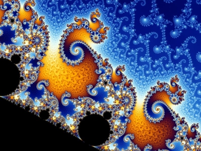
The self-similarity at all scales of the water at the critical point is analogous to that seen in fractals, such as this Mandelbrot set, created by Wolfgang Beyer. Of course the positions of the features of the Mandelbrot set are entirely determined by the mathematical function that generates it. Whereas the exact positions of the water droplets and bubbles of steam are down to chance and statistical mechanics. You can read more in the article Unveiling the Mandelbrot set.
The scales fall from our eyes
Very similar behaviour can be seen in materials such as iron, where the second order phase transition occurs at the Curie temperature. Above this temperature, 771 degrees Celsius, iron loses its inherent magnetism. As the iron cools below this temperature it will spontaneously become magnetic, the magnetic field it creates becoming stronger the cooler the material.
Magnetic behaviour is due to the tiny magnetic fields produced by individual electrons in the material. It can be modelled as follows. If you think of each electron in iron as arranged in a lattice, then the material is magnetic if more than half of the electron spins pointed the same way, either up or down. The more electrons point the same way, the stronger the magnetic field. Electrons in iron tend to align themselves with their neighbours, creating a magnet, as being similarly aligned takes less energy. As the temperature of the material increases, the electrons have more energy to overcome this natural tendency. They jiggle about more, making them more likely to randomly flip in direction, explaining why the magnetism decreases as the temperature rises. (This trade-off between the low-energy ordered state and the random jiggling at higher energies lies at the heart of statistical mechanics. You can read more in Secret symmetry and the Higgs boson.)
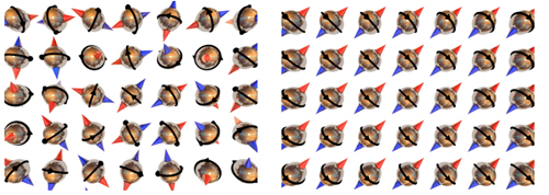
Left: Schematic depiction of the atoms in a ferromagnet. Left: The symmetrical phase above the Curie temperature where all the magnetic fields of the atoms are randomly oriented. Right: The asymmetrical phase below the Curie temperature where the magnetic fields of all the atoms are aligned in the same direction. Image: Nick Mee, taken from his Plus article about the Higgs boson.
This explains the gradual loss of magnetism with increased temperature. However, to understand the sudden loss of magnetism at the Curie temperature, you have to consider all the scales of the problem. Above this temperature, any block of electrons in the lattice with more than half the spins pointing one way, will contain a smaller block with the majority pointing the other way, and this swapping of polarity continues for smaller and smaller blocks all the way down to individual electrons on the lattice. "Thus an ocean of spins that are mostly up may have within it an island of spins that are mostly down, which in turn surrounds a lake of up spins with an islet of down spins," as Wilson poetically put it. "The progression continues to the smallest possible scale: a single spin."
The need to account for behaviour at so many different scales made a mathematical description of the physics in second order phase transitions, also called critical points (such as critical opalescence and a ferromagnet's Curie temperature) incredibly complex, requiring a huge number of variables to characterise the state of the material. For example, to describe the behaviour of iron at the Curie temperature, you apparently would need to know the direction of the spin of every electron in the material.
In 1966 Leo Kadanoff, an American condensed matter physicist, suggested a very intuitive averaging process as a way to overcome this difficulty. Kadanoff started with the lattice of electrons described above, with a spacing of, say, L=1 unit between the electrons. He then reduced the complexity of the problem by dividing the lattice into 3x3 blocks by treating each group of 9 blocks as a single element. The spin of this element was defined to be the same as the majority of spins of the electrons it contained. If the spin of the majority of the electrons in this block pointed up, then the block would represented by single spin also pointing up, and vice versa. This defined a new lattice of spins, with elements (the blocks) spaced L units apart. Then he defined larger blocks containing 3x3 of each of these elements in the same way, producing a lattice of spins with elements L units apart. This process of using an increasingly coarse-grained picture of the system could be repeated. If you think of the spacing of the lattice as analogous to the "degree of resolution" on the microscope that you are using to observe the material, then Kadanoff's block spin process was like zooming out, again and again.
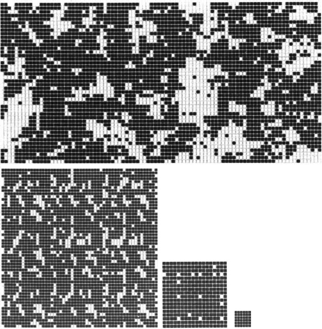
The progression Kadanoff's block spin method for a metal below the Curie temperature. The top lattice is the original metal below the Curie temperature with black indicating the spin of the electron pointing up, white indicating the spin is pointing down. The lower lattices showing the subsequent steps in the averaging process, with the up spins (black squares) becoming dominant at larger scales.
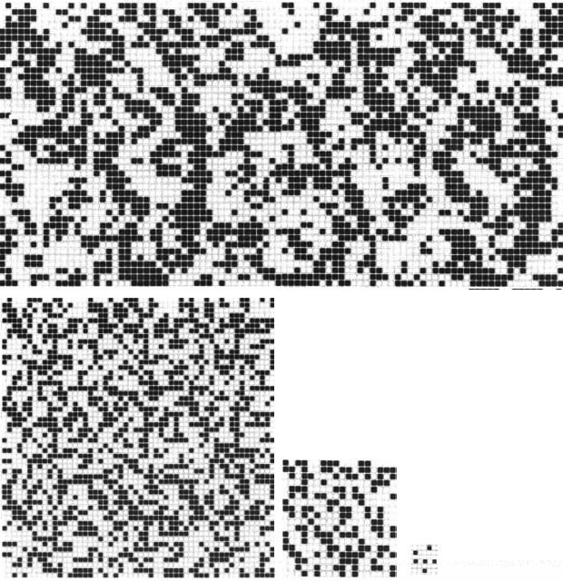
The progression of the block spin method for a metal above the Curie temperature. The top lattice is the original metal, with the lower lattices showing the subsequent steps in the averaging process. Above the Curie temperature no direction of spin is dominant on any scale.
For example, suppose we applied Kadanoff's approach to a piece of iron below the Curie temperature (the images above on the left). Then, although there might be some differences in alignment at small scales (the top lattice), as we zoom out (and L, the distance between the units in the lattice, grows) these differences will average out (the lower lattices). For large values of L the spins of all these larger blocks will point in the same directions. If we instead use this approach for a piece of iron that is above the Curie temperature (the images on the right), the differences in alignment of the blocks will remain at every length scale, from individual electrons to the largest blocks. Kadanoff's approach simplified the mathematics, so that it was finally possible to to predict the behaviour of these materials, accurately matching the data measured in experiments.
This block spin method from statistical physics provides a way of zooming in and out of a system to examine it on many scales. And it turned out to be just the idea that was needed to tame the strange quantum world. Find out how in the second part of this article.
About this article
Marianne Freiberger and Rachel Thomas are Editors of Plus. They are very grateful to David Kaiser, a historian of physics at Massachusetts Institute of Technology, for an illuminating conversation and his excellent book Drawing theories apart. But they owe most of their tentative understanding of quantum field theory to Jeremy Butterfield, a philosopher of physics at the University of Cambridge, and Nazim Bouatta, a Postdoctoral Fellow in Foundations of Physics at the University of Cambridge. Many thanks to them for their many patient explanations and help in writing this article.
Comments
lschudel
I really enjoyed this article and I will be reading the literature that you recommend. Just wanted to let you know that I appreciate your work.