How can maths fight an epidemic?

Brief summary

The SIR model is the basis most disease modellers use to understand the spread of disease through a population. In its most basic form this model assumes that people in a population are either susceptible to the disease (S), infected with the disease (I) or recovered (R) from the disease.

Mathematical equations describe how people move between being susceptible, infected or recovered. These equations depend on the transmission rate for the disease and also the recovery rate. The model can be used to simulate an epidemic on a computer.

The basic idea behind using maths to try and predict how an infectious disease will spread is surprisingly straight-forward. Suppose you have observed that the number of people infected with a particular disease doubles every three days. Then it’s quite easy to work out that, if today we have $x$ cases and this trend continues, then we will have

$2x$ cases in 3 days,

$4x$ cases in 6 days,

$8x$ cases in 9 days

and, generally, $2^ nx$ in 3 $n$ days. That’s the steep growth that can lead to a disease spreading very quickly.

This extrapolation, simple as it may be, highlights the basic ingredients of a model: a mathematical expression which describes the general nature of the change that will happen over time and parameters which pin down the exact shape of the change. In our example we have exponential growth over time, and the steepness of this growth is decided by the parameter of the doubling time, which is 3 days.

The SIR model

Let $S$ denote the number of susceptible people, $I$ the number of infected people, and $R$ the number of recovered people. The equations for the SIR model are

$\displaystyle \frac{dS}{dt}$	$\displaystyle =$	$\displaystyle - \beta SI$
$\displaystyle \frac{dI}{dt}$	$\displaystyle =$	$\displaystyle \beta SI - \nu I$
$\displaystyle \frac{dR}{dt}$	$\displaystyle =$	$\displaystyle \nu I$

Here $\beta$ is the transmission rate and $\nu$ is the recovery rate. The expressions $d/dt$ represent the rate of change over time, so $dS/dt$ means the rate of change of the number of susceptibles over time.

The number $R_0= \beta /\nu N,$ where $N$ is the size of the population, is called the basic reproduction number of the disease.

You can find out more about the SIR model in this article.

If you want longer term predictions and to simulate the impact of interventions in detail, you need a more sophisticated model. Different models are designed for different purposes, such as making short term predictions, long term predictions, or simulating the effect of particular interventions such as school closures. But although models differ, they tend to be built around an approach that has been around since the 1910s: the SIR model.

To get the general idea behind the SIR model, imagine a population of people in which everyone is either susceptible to a disease (S), infected (I), or recovered (R) and therefore immune. The way people pass from the S class into the I class, and then from the I class into the R class, is described by mathematical equations. These equations depend on the transmission rate for the disease and also the recovery rate. You start the model off with only a small proportion of the population in the I class, and then let it evolve over time, seeing how the disease spreads and then subsides as people recover and become immune.

Although simple, the SIR model gives good predictions for simple populations, such as students at a boarding school, which form a closed group relatively isolated from the rest of the population. When it comes to more complex populations you can link up many individual SIR models representing different geographical locations and sub-populations, including for example individual towns or schools.

Contacts are key

Back to the Epidemiology for beginners collection.

What is hugely important in this context are people's contact patterns: who meets whom and how frequently. Information on this comes from social mixing studies. An example is a large-scale citizen science project which ran in 2018 as a collaboration between the BBC and a research team headed by Julia Gog, an epidemiologist at the University of Cambridge. Here people were asked to download an app which tracked their movements and asked them to keep track of the people they met (all suitably anonymised). Such contact data is represented mathematically by arrays (matrices) of numbers (see the figure below) which are built into the model.

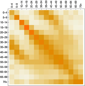
A contact matrix displaying average contacts between different age groups. Darker shades indicate more contacts (here the colours are used instead of numbers to make the matrix easier to understand). The figure is from the paper Contagion! The BBC Four Pandemic – The model behind the documentary. (Used by permission.)

To see how a particular change, such as school holidays, might affect the spread of the disease, you adapt the contact data accordingly by removing or scaling down parts of it that relate to the change, such as contacts between school-aged people. This, put simply, is how epidemiological modelling works.

But are the models right?

There isn't just one epic model designed to represent the whole of the UK, Europe, or even the entire world. Instead, there are many different ones designed to do different things and, although the compartmental approach of the SIR model is a ruling paradigm, models can still be different in their nature. Some are completely deterministic, others contain a degree of randomness, some are designed to run just once to demonstrate the role of one particular factor, others are run many times to get ranges of predictions in the face of uncertainty.

The big question is whether the models are realistic. Although the dynamics of different diseases can be similar, there can also be important differences. One is that different diseases can have different latent periods in which a person can have the infection without showing any symptoms. "For 'flu maybe you get a few hours of that, but for [COVID-19] it can be a few days," says Gog. In terms of the model this means moving into the world of SEIR, where E stands for "exposed": people in this class have the infection but no symptoms yet. The E class can be split further into those who are infectious to others and those who aren't. "All models are approximations, and for 'flu you can often get away with SIR, depending on what you are trying to address with the model. But ignoring the latent period for COVID-19 would be a much worse approximation, especially if making short-term predictions, so usually it does need to be considered," says Gog.

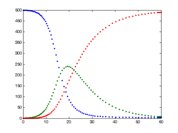
This is the typical output from a simple SIR model. The number of susceptible people is shown in blue, the number of infected in green, and the number of recovered in red.

When the disease you are looking at is novel, for example when a new virus emerges in a human population, there are also usually plenty of other things we don't know. "Inferring [missing information] from [the available] data [can be] very hard. You just try and do your best to extrapolate from limited information." When there isn't enough information, modellers decide which of the unknowns are most important to resolve in order to remove uncertainty — making such calls is a critically important aspect of modelling.

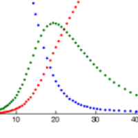
The importance of any one parameter can depend on exactly what you are trying to do. "To predict how many cases there are going to be tomorrow you don't need to know many things. It's almost exponential [at the start of an epidemic]," says Gog. "But to make a prediction about whether there is going to be a second [peak of the epidemic] you need to know some really very different things."

An important number for longer term predictions is the basic reproduction number of a disease (often denoted as $R_0$ ): the number of people an infectious person will infect on average, assuming that everyone in the population is susceptible to the disease (it is related to the transmission rate, see the box above). For seasonal strains of flu, it lies between 0.9 and 2.1, and for measles it is a whopping 12 to 18. Modellers will often run their model for each of a range of possible values, coming up with a range of corresponding predictions. (You can see an example in this article, where a model is run several times to reflect different levels of transmissibility.)

But even with imperfect information, modelling predictions are not just stabs in the dark especially if they account for and present the range of uncertainty. Good models comprise all the relevant information we do have. Good modellers keep careful track of the limitations of their models and the uncertainties within them, often including ranges of possible parameter values, which then lead to ranges of predictions: ranges of possible future scenarios that may occur under different intervention strategies. The predictions won't be perfect, but they are the best we can do with the information we have.

About this article

Julia Gog is Professor of Mathematical Biology at the University of Cambridge and co-lead of the JUNIPER network. Gog is also a member of the Scientific Pandemic Infections group on Modelling (SPI-M), an advisory group of the Department of Health and Social Care which provides expert advice to the UK government based on infectious disease modelling and epidemiology and fed results into the Scientific Advisory Group for Emergencies (SAGE) during the COVID-19 pandemic.

Marianne Freiberger, Editor of Plus, interviewed Julia Gog on March 24, 2020

This article is part of our collaboration with JUNIPER, the Joint UNIversities Pandemic and Epidemiological Research network. JUNIPER is a collaborative network of researchers from across the UK who work at the interface between mathematical modelling, infectious disease control and public health policy. You can see more content produced with JUNIPER here.